Gradient Scalability and Taylor Surrogation of Quantum Cost Landscapes
Pith reviewed 2026-05-21 23:42 UTC · model grok-4.3
The pith
A Linear Clifford Encoder produces constant-scaling gradients near Clifford circuits while keeping super-polynomial complexity outside classically simulable regions.
A machine-rendered reading of the paper's core claim, the machinery that carries it, and where it could break.
Core claim
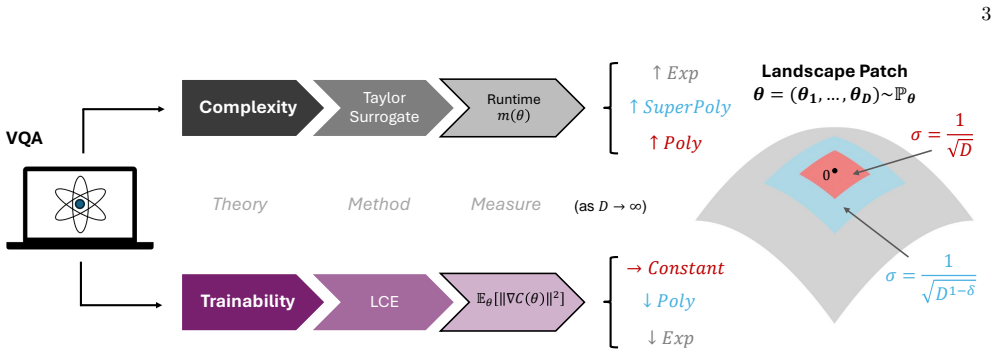
Beyond previously established classically simulable regions, variational quantum algorithm complexity is at least super-polynomial, and the Linear Clifford Encoder ensures constant-scaling gradients within landscape regions close to Clifford circuits, with numerical evidence indicating polynomial rather than exponential gradient decay in the transition to these harder regions.
What carries the argument
The Linear Clifford Encoder, a classically efficient ansatz modifier that enforces constant-scaling gradients near Clifford circuits.
If this is right
- Gradients remain constant in scale near Clifford circuits after the ansatz modification.
- Computational complexity stays at least super-polynomial outside the regions that admit efficient classical simulation.
- In the transition zone, gradients can decay polynomially instead of exponentially while complexity remains hard.
- Non-vanishing gradients and super-polynomial complexity may coexist in certain landscape instances.
Where Pith is reading between the lines
- These transition zones could be targets for hybrid algorithms that combine classical pre-processing with quantum evaluation.
- Extending the Taylor surrogate to cover more of the transition region might yield practical simulation tools for near-term devices.
- The findings weaken the strict link between avoiding barren plateaus and full classical simulability, suggesting the need for refined complexity measures.
Load-bearing premise
The Linear Clifford Encoder keeps gradients from vanishing near Clifford circuits without lowering the landscape complexity below super-polynomial outside the previously simulable areas.
What would settle it
Direct computation showing that gradients still vanish exponentially with system size in the modified landscapes even near Clifford circuits would refute the constant-scaling claim.
Figures


read the original abstract
Variational Quantum Algorithms are promising candidates for near-term quantum computing, yet they face scalability challenges due to barren plateaus, where gradients vanish exponentially relative to system size. Recent conjectures suggest that avoiding these plateaus might inherently lead to classical simulability, thereby limiting the opportunities for quantum advantage. In this work, we advance the theoretical understanding of the relationship between gradient scalability at initialization and the computational complexity of variational quantum algorithms. We first present the Taylor surrogate, a classical simulation technique that matches Pauli path runtime guarantees on near-Clifford regions while offering runtime advantages in specific regimes. Leveraging this surrogate, we prove that beyond previously established classically simulable regions, the computational complexity is at least super-polynomial. Next, we introduce the Linear Clifford Encoder, a classically efficient ansatz modifier that ensures constant-scaling gradients within landscape regions close to Clifford circuits. Finally, numerical experiments on these modified landscapes provide preliminary empirical evidence of a transition zone where constant-scaling gradients may decay polynomially in super-polynomially complex regions rather than exponentially. These findings suggest speculative instances where non-vanishing gradients and super-polynomial complexity could potentially coexist, vindicating the need for future formal proofs.
Editorial analysis
A structured set of objections, weighed in public.
Referee Report
Summary. The manuscript introduces the Taylor surrogate, a classical simulation technique matching Pauli path runtime guarantees near Clifford circuits with potential runtime advantages in specific regimes. It proves that beyond previously established classically simulable regions, the computational complexity of variational quantum algorithms is at least super-polynomial. The work then defines the Linear Clifford Encoder, a classically efficient ansatz modifier ensuring constant-scaling gradients near Clifford circuits, and presents numerical experiments on modified landscapes providing preliminary evidence of a transition zone in which constant-scaling gradients decay polynomially rather than exponentially within super-polynomially complex regions.
Significance. If the central claims are substantiated, the results would offer a concrete counter-example to conjectures that non-vanishing gradients necessarily imply classical simulability, thereby opening a speculative window for quantum advantage in variational algorithms. The Taylor surrogate is a positive contribution with explicit runtime comparisons, and the numerical identification of a polynomial-decay transition zone, while preliminary, supplies falsifiable empirical signatures that can guide future proofs. The overall framing strengthens the theoretical link between gradient scaling at initialization and complexity class.
major comments (3)
- [Linear Clifford Encoder definition and complexity analysis] Linear Clifford Encoder section: the central claim that this classically efficient modifier preserves super-polynomial complexity outside previously simulable regions while enforcing constant gradient scaling is load-bearing for the transition-zone interpretation, yet the manuscript supplies no explicit reduction or simulation argument showing that the encoder does not inadvertently introduce additional structure permitting efficient classical approximation or polynomial-time simulation.
- [Complexity proof after Taylor surrogate] Proof of super-polynomial complexity (following the Taylor surrogate introduction): the argument that complexity remains at least super-polynomial beyond simulable regions relies on the surrogate matching Pauli-path guarantees, but it is not shown how the surrogate avoids reducing the effective complexity class or how the complexity lower bound is independent of the surrogate's own fitting parameters.
- [Numerical experiments and transition-zone evidence] Numerical experiments section: the reported transition zone with polynomial rather than exponential gradient decay is the key empirical support, but the text provides no quantitative definition of the transition (e.g., fitting procedure, system-size scaling, or statistical test distinguishing polynomial from exponential), nor details on ansatz depth, number of samples, or error analysis, rendering the evidence difficult to assess or reproduce.
minor comments (2)
- [Abstract and Taylor surrogate runtime discussion] The abstract states that the surrogate 'matches Pauli path runtime guarantees'; a direct runtime comparison table or equation would clarify the claimed advantage in specific regimes.
- [Ansatz modification description] Notation for the Linear Clifford Encoder should include an explicit statement of how the encoder is applied to the original ansatz (e.g., as a pre- or post-processing layer) to avoid ambiguity in the numerical setup.
Simulated Author's Rebuttal
We thank the referee for their constructive comments and for recognizing the potential significance of our results. We address each of the major comments in detail below, indicating the revisions we plan to make to strengthen the manuscript.
read point-by-point responses
-
Referee: [Linear Clifford Encoder definition and complexity analysis] Linear Clifford Encoder section: the central claim that this classically efficient modifier preserves super-polynomial complexity outside previously simulable regions while enforcing constant gradient scaling is load-bearing for the transition-zone interpretation, yet the manuscript supplies no explicit reduction or simulation argument showing that the encoder does not inadvertently introduce additional structure permitting efficient classical approximation or polynomial-time simulation.
Authors: We agree that an explicit argument for complexity preservation is important for the claim. The Linear Clifford Encoder is defined as a modification that applies a linear map over Clifford basis states to the variational parameters, which is classically computable but does not simplify the non-Clifford components of the original ansatz. We will add a new paragraph in the section providing a high-level argument that any efficient classical simulation of the modified circuit would imply one for the original, thus preserving the super-polynomial hardness. This will be a partial revision as a full formal reduction may require additional technical work. revision: partial
-
Referee: [Complexity proof after Taylor surrogate] Proof of super-polynomial complexity (following the Taylor surrogate introduction): the argument that complexity remains at least super-polynomial beyond simulable regions relies on the surrogate matching Pauli-path guarantees, but it is not shown how the surrogate avoids reducing the effective complexity class or how the complexity lower bound is independent of the surrogate's own fitting parameters.
Authors: The Taylor surrogate is employed solely as a tool to analyze the landscape near Clifford circuits and does not alter the underlying variational circuit for the complexity analysis. The super-polynomial complexity lower bound is derived from a direct reduction to known hard instances of variational quantum algorithms outside the simulable regime, independent of the surrogate's approximation parameters. We will revise the proof section to explicitly state this independence and clarify that the surrogate is not used in establishing the lower bound itself. revision: yes
-
Referee: [Numerical experiments and transition-zone evidence] Numerical experiments section: the reported transition zone with polynomial rather than exponential gradient decay is the key empirical support, but the text provides no quantitative definition of the transition (e.g., fitting procedure, system-size scaling, or statistical test distinguishing polynomial from exponential), nor details on ansatz depth, number of samples, or error analysis, rendering the evidence difficult to assess or reproduce.
Authors: We acknowledge the need for more rigorous presentation of the numerical results. In the revised manuscript, we will include: (1) a quantitative definition of the transition zone based on fitting the gradient norm scaling to both polynomial (O(1/n^k)) and exponential (O(exp(-c n))) forms and comparing goodness-of-fit via R^2 or AIC; (2) specification of ansatz depths used (typically 4-12 layers); (3) number of samples per data point (at least 5000 shots per gradient estimate); and (4) error analysis using standard deviation over 10 independent runs. These additions will make the evidence more reproducible and allow better assessment of the polynomial decay claim. revision: yes
Circularity Check
No significant circularity; derivation relies on introduced techniques and external benchmarks
full rationale
The paper defines the Taylor surrogate as a new classical simulation method matching Pauli-path guarantees near Clifford regions and leverages it to prove super-polynomial complexity outside previously simulable areas. It separately introduces the Linear Clifford Encoder as a classically efficient ansatz modification that enforces constant-scaling gradients near Clifford circuits by construction of the modifier itself. Numerical experiments then examine the resulting modified landscapes for a transition zone. No quoted equations or steps reduce the central claims to fitted inputs, self-definitions, or load-bearing self-citations; the complexity lower bound and gradient scaling are established via the new surrogate and encoder definitions plus external simulability results, making the chain self-contained against benchmarks.
Axiom & Free-Parameter Ledger
free parameters (1)
- Numerical experiment parameters
axioms (2)
- domain assumption Near-Clifford regions admit efficient classical simulation with Pauli path guarantees
- ad hoc to paper Linear Clifford Encoder preserves constant gradient scaling without changing complexity class
invented entities (2)
-
Taylor surrogate
no independent evidence
-
Linear Clifford Encoder
no independent evidence
Reference graph
Works this paper leans on
-
[1]
Theorem 1) to establish a constant lower bound
Constant Gradient Lower Bound in Small Patches Having derived a lower bound for the expected squared gradient norm with an error term perturbing a given component (∂θk C)(0), we combine this result with the LCE (cf. Theorem 1) to establish a constant lower bound. In particular, this guarantees a tight escape from barren-plateaus as per Eq. (9): Corollary ...
-
[2]
This outcome holds with probability one for all observablesH as defined in Eq
Polynomial Gradient Lower Bound beyond Small Patches Utilizing the LCE method in conjunction with Lebesgue measure theory and previous results, we are ready to rigorously show that barren plateaus are mitigated beyond the threshold σ = O(D−1/2), a landscape patch lacking any known classical surrogate [18]. This outcome holds with probability one for all o...
-
[3]
Worst-Case Error: m = m(θ) is a deterministic function of a fixed configuration θ ∈ [−π, π]D
-
[4]
Mean-Squared Error: m = m(Pθ) is defined probabilistically based on an initialization distribution Pθ
-
[5]
Worst-Case Error Analysis The following lemma quantifies the (deterministic) worst-case error of the approximation Cm(θ) ≈ C(θ) as a function of θ. Lemma 7. Consider an expectation of the form Eq. (E1) with a variational ansatz U(θ) involving D ≥ 1 parameters, and suppose we simulate it classically using the Taylor series Cm(θ) defined in Eq. (D9). Let θ ...
-
[6]
Mean-Squared Error Analysis Next, we quantify the mean squared error of the approximation Cm(θ) ≈ C(θ) with respect to the local distribution Pθ ∈ {N (0, σ2ID), Unif([−σ, σ]D)} for some σ > 0. However, we first require the following counting argument to conclude with the result: Lemma 10. Let m = O(1) be of constant order, i.e., independent of D. Then, X ...
-
[7]
The Complexity Class of LCE Hamiltonians In order to successfully mitigate barren plateaus of arbitrarily expressive PQC unitaries U(θ) on large parameter landscape patches with LCE (cf. Theorem 5), we are restricted to the class of observables, H = X i∈I ciPi with ∥H∥ = O(1) and ci0 = Ω(1) for some i0 ∈ I , (J1) where I ⊂ { I, X, Y, Z }⊗N \{I2N } is an a...
-
[8]
Deterministic Worst-Case Simulation Complexity The next parts leverage the results of the previous section, and focuses on the computational complexity of sim- ulating the cost function C(θ) in Eq. (E1) with the help of the Taylor surrogate Cm(θ) in Eq. (D9). We shall use Time Cm(θ) to denote the time complexity of evaluating Cm(θ), which is, by definitio...
-
[9]
Probabilistic Mean-Squared Simulation Complexity Next, we use the mean-squared error analysis in order to determine the Gaussian/uniform initialization strategy Pθ that covers the largest landscape patch where Taylor surrogating the cost C(·) remains polynomially efficient. Theorem 4. Consider an expectation of the form in Eq. (E1) with a variational ansa...
-
[10]
[18], as long as the patch is sufficiently small: Corollary 3
Complexity Comparison with the Pauli Path Surrogate We conclude our complexity analysis by showing that our Taylor surrogate outperforms the Pauli path surrogate employed by Lerch et al. [18], as long as the patch is sufficiently small: Corollary 3. Consider an expectation of the form in Eq. (E1) with a variational ansatz U(θ) involving D ≥ 1 parameters, ...
-
[11]
Efficient Recursive Classical Implementation In a practical implementation of our simulation strategy, one has to iterate over the summation {∥α∥1 < m } in Eq. (D9). Concretely, we are interested in finding all multi-index combinations in the set: Am,D := {α = (α1, . . . , αD) ∈ ND 0 : ∥α∥1 < m}. (J58) When using a for-loop naively, one will be confronted...
-
[12]
Gradient Scaling Experiments We repeat the initial gradient scaling experiments (cf. Figs. 5 and 6) comparing all models considered in this work: mHEA, fHEA, and rPQC (defined in Appendix C). Fig. 13 illustrates the expected behavior of the initial gradient norm at θ = 0 employing various PQC models with L = 1 layer. Gradients are computed analytically vi...
-
[13]
Furthermore, we address the issue of finite sampling noise [58]
VQE Optimization with different Learning Rates and Finite Sampling Noise Here, we demonstrate that LCE is effective for smaller learning rates in vanilla gradient descent. Furthermore, we address the issue of finite sampling noise [58]. We use a small number of finite shots to evaluate the gradients in order to emphasize that LCE remains relevant for near...
-
[14]
VQE Optimization of the Heisenberg Model In this experiment, we leverage the benchmarked initial gradient scaling statistics to optimize the VQE of the N = 12 qubit Heisenberg model [59], HHeisenberg := N −1X j=1 {XiXi+1 + YiYi+1 + ZiZi+1} . (K1) Eq. (K1) defines a local observable and thus is less prone to the barren plateau problem [57]. In order to inc...
work page 2000
discussion (0)
Sign in with ORCID, Apple, or X to comment. Anyone can read and Pith papers without signing in.