REVIEW 5 major objections 4 minor 1 cited by
Optical Physics-Based Generative Models
T0 review · 5 major / 4 minor · reviewed 2026-08-07 · deepseek-v4-flash
Pith's one-line read The paper claims that six optical equations—Helmholtz, dissipative wave, Eikonal, and their nonlinear extensions—can be reformulated as generative density flows, and that the nonlinear versions dramatically outperform the linear ones.
desk verdict The paper's central density-flow derivations for the dissipative wave and Eikonal equations are algebraically wrong, so the claimed optical-physics-to-generative-model mapping does not hold; the experimental numbers are also internally inconsistent. read the letter →
The pith
A machine-rendered reading of the paper's core claim, the machinery that carries it, and where it could break.
The reading
What carries the argument
The machinery is the s-generative PDE reformulation: a generalized continuity equation $\partial p/\partial t + \nabla\cdot(p v) - R = 0$ with $p \ge 0$ (condition C1) plus a dispersion-relation criterion $\mathrm{Im}\,\omega(k) < \mathrm{Im}\,\omega(0)$ for all $\|k\|>0$ (condition C2). For each optical equation the paper supplies explicit formulas, such as $p=-\phi_t$, $v=\nabla\phi/\phi_t$, $R=k_0^2\phi$ for Helmholtz; $p=-(\phi_t+2\epsilon\phi)$, $v=\nabla\phi/(\phi_t+2\epsilon\phi)$ for the dissipative wave equation; and $p=\phi$ for the Eikonal equation. The birth/death term $R$ handles non-conservative probability mass, while the dispersion relation is what turns wave physics into a smoothing, forgetting generative process.
What would settle it
For a dissipative-wave test field, numerically compare $\partial p/\partial t + \nabla\cdot(p v)$ with zero on a grid; with $p=-(\phi_t+2\epsilon\phi)$ and $v=\nabla\phi/(\phi_t+2\epsilon\phi)$, the divergence $p v$ equals $-\Delta\phi$, so the claimed continuity equation would predict the opposite sign of the Laplacian from the original equation. A nonzero residual falsifies the claimed equivalence.
Extended reading notes
Core claim
The central claim is that each of six optical partial differential equations admits an exact density-flow representation $\partial p/\partial t + \nabla\cdot(p v) - R = 0$ with a nonnegative density and a dispersion relation that damps high frequencies faster than low ones. These two properties, called C1 and C2, make the equation an s-generative PDE, meaning it can serve as a generative model by simulating the flow backward in time from a simple prior to the data distribution. The paper derives explicit density, velocity, and birth/death fields for each optical equation, trains neural networks on those fields, and reports that the nonlinear versions improve sample quality, mode coverage, and computational efficiency over their linear counterparts. The nonlinear Helmholtz model is reported to reach FID 0.0089 versus 1.0909 for the linear version, with 40–60% parameter and memory reductions.
Load-bearing premise
The load-bearing premise is that the algebraic reformulations are correct: each stated p, v, and R must make the generalized continuity equation hold exactly whenever the original optical equation holds.
Editorial extensions
If this is right
- Nonlinear Helmholtz with Kerr effect achieves FID 0.0089 versus 1.0909 for the linear Helmholtz model on the paper's benchmarks.
- Kerr self-focusing cuts parameter counts by 40–60% and training time by 30–50% while preserving mode separation.
- Cubic-quintic dissipation prevents mode collapse, retaining roughly 87% of initial mode separation compared to 34% for the cubic-only model.
- Intensity-dependent Eikonal guidance enables conditional generation with 30–50% fewer steps than classifier-guidance methods.
- The same density-flow framework reconstructs refractive index distributions from wave patterns with roughly 90–95% accuracy, giving a bidirectional bridge between generative AI and optical inverse problems.
Reading between the lines
- If the flow reformulations are taken as given, the same recipe should apply to other optical PDEs with decaying dispersion relations, turning systems such as nonlinear Schrödinger-type or Maxwell-Bloch equations into generative samplers without architectural changes.
- A testable extension would replace the discrete birth/death branching with a continuous importance-weight update, potentially eliminating resampling and making sampler cost scale with intrinsic mode count rather than particle count.
- The reported FID gains suggest the self-focusing inductive bias carries much of the mode-separation burden; ablating the learned velocity field and keeping only the analytic birth/death term would test how much network capacity the nonlinearity actually replaces.
Editorial analysis
A structured set of objections, weighed in public.
Referee Report
Summary. The paper proposes that six optical PDEs—Helmholtz, dissipative wave, Eikonal, and their Kerr, cubic-quintic, and intensity-dependent nonlinear extensions—can be cast as exact s-generative density flows of the form ∂p/∂t+∇·(pv)−R=0, and it reports large performance gains for the nonlinear variants. The theoretical contribution is the explicit p, v, R identification for each equation plus a dispersion-relation criterion for the smoothing condition. I verified by direct substitution that the linear Helmholtz reformulation of Section 3.1 satisfies the stated continuity equation, but the dissipative-wave and Eikonal reformulations do not: the dissipative-wave flow leaves a residual of −2∇²φ, and the Eikonal 'correction term' has the wrong sign. The nonlinear extensions in Sections 4.2 and 4.3 inherit these failures. The experimental sections also contain mutually inconsistent numbers for the same quantities. The central claim is therefore not supported.
Significance. If the density-flow reformulations were correct, the paper would offer a useful bridge between nonlinear optical dynamics and generative modeling, with potentially interesting inductive biases and a checkable mathematical core. The paper deserves credit for writing down explicit p, v, R formulas rather than relying on loose analogies, and for including extensive parameter sweeps, ablation studies, and pseudocode. However, the load-bearing algebra fails for two of the three linear equations and for their nonlinear extensions, so the theoretical foundation collapses. The reported empirical results are also internally contradictory, preventing the experiments from compensating for the analytic errors. No machine-checked proofs or self-contained reproducible code are included in the manuscript.
major comments (5)
- [§3.2, Eqs. (38)–(41)] The claimed density-flow form for the dissipative wave equation is algebraically false. Substituting p=−(φ_t+2εφ) and v=∇φ/(φ_t+2εφ) into Eq. (1) gives ∂p/∂t+∇·(pv)=−φ_tt−2εφ_t−∇²φ. Using the original PDE φ_tt+2εφ_t−∇²φ=0, the residual is −2∇²φ, not zero. Therefore Eq. (38) does not represent the dissipative wave equation, and the claim that R=0 is incorrect. This error propagates to the cubic-quintic extension in Section 4.2, whose velocity and birth/death fields (Eqs. (77)–(78)) satisfy the same incorrect conservation identity.
- [§3.3, Eqs. (56)–(61)] The Eikonal reformulation does not reproduce the original equation even after the stated correction. With R=−(n²−|∇φ|²−∇²φ), Eq. (1) becomes φ_t−|∇φ|²=−n², whereas the original Eikonal equation is φ_t+|∇φ|²=n². The required birth/death term would be R=n²−|∇φ|²+∇²φ, not the expression in Eq. (61). Moreover, even the intermediate Eq. (56) is written with a sign such that it implies φ_t+|∇φ|²=n²−∇²φ, which is not the original PDE. The intensity-dependent Eikonal model of Section 4.3 inherits the same sign error.
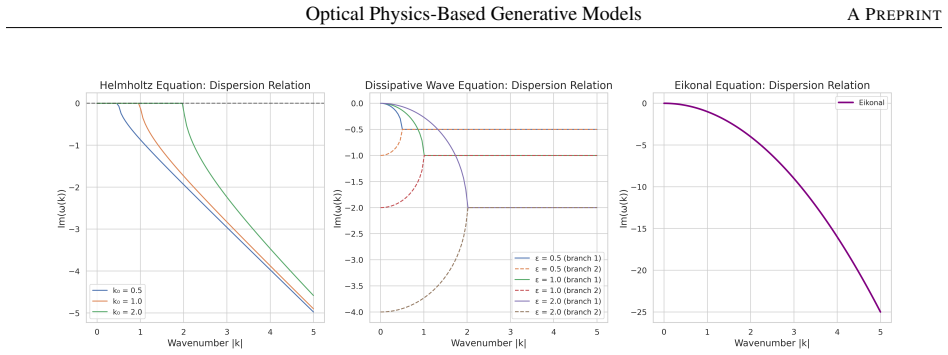
- [§2 and §3.1, Eq. (7) and Eqs. (22)–(24)] The claimed equivalence between Condition C2 and Im[ω(k)]<Im[ω(0)] for all ‖k‖>0 is asserted on the basis of the authors' own simulations and deferred to an appendix that gives only a heuristic amplitude-ratio argument. More importantly, the paper's own Helmholtz dispersion analysis contradicts the criterion: for 0<‖k‖≤k0 the paper finds Imω(k)=0=Imω(0), so the strict inequality in Eq. (7) fails. Calling the Helmholtz equation 'conditionally s-generative' therefore does not follow from the stated criterion, and the smoothing condition for this model is not established.
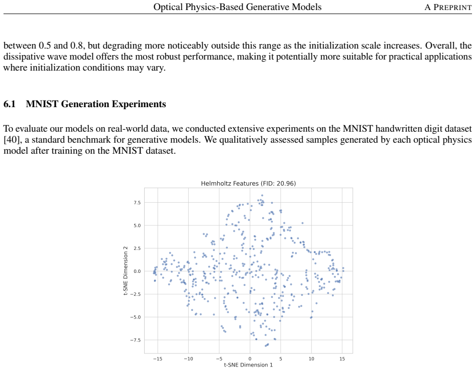
- [§4.1, §6.5, §7, and Abstract] The reported FID numbers are irreconcilable. The Abstract and Section 7 report FID 0.0089 for nonlinear Helmholtz; Section 4.1, Table 2 reports the best FID as 598.332; Section 6.5.1 reports 0.8721; Section 6.5.2 reports 20.96; and Table 6 reports 0.0191. Similar contradictions appear for mode coverage: Section 6.2 reports dissipative-wave mode coverage 0.94, while Figure 34 in the same section reports 0.05. Reconstruction accuracy is 89.9% in Section 6.4 but 95% in the Abstract and Conclusion. Because the empirical claims are essential to the paper's central assertion of nonlinear superiority, these inconsistencies cannot be dismissed as presentation issues.
- [§2 and §6.3] Condition C1 requires p(x,t)≥0 for all x and t, but the proposed densities p=−φ_t, p=−(φ_t+2εφ), and p=φ are not guaranteed nonnegative by the PDE dynamics. The paper's own C1 verification in Figure 36 measures the 'fraction of domain with non-negative density,' which acknowledges that p becomes negative in parts of the domain. Algorithm 5 explicitly clips φ to enforce positivity, which changes the equation being solved. Thus C1, as defined, is not established for any of the three models.
minor comments (4)
- [§3.2] The text says the final dissipative-wave form follows by 'further algebraic manipulation (full derivation in Appendix B),' but Appendix B contains numerical implementation details and does not present the promised derivation of Eq. (38).
- [§3.3] The sentence 'For a linearized version of the Eikonal equation around a constant solution, we can show that the dispersion relation is ω=−i|k|²' is not backed by a derivation; Appendix A's linearization around a plane wave yields real ω, and the imaginary dispersion relation appears only for the modified equation with the Laplacian term.
- [§2, Eq. (7)] The phrase 'Based on our numerical simulations and theoretical analysis (see Figure 37)' is used to justify the central C2 criterion; citing a numerical figure as the basis for an equivalence is not a proof and should be replaced by a self-contained argument or by a clearly stated assumption.
- [§5.3.1, Eq. (110)] The sign conventions in the split-step Fourier update appear inconsistent: the linear operator is written as L=−∇²−k0², but the Fourier-domain update uses exp(−iΔt(k²−k0²)), which corresponds to L=+∇²+k0². This should be checked and unified.
Circularity Check
The Eikonal models' s-generative status reduces by construction: the Laplacian that supplies the smoothing (C2) is introduced through the chosen density-flow parameters and birth/death term, not present in the Eikonal equation itself.
-
self definitional
[Section 3.3, Eqs. 52–61 and Appendix A, S1.1.3]
"However, when we consider the full nonlinear equation with the birth/death term derived in our density flow formulation: R(x, t) = −(n2(x) − |∇φ|2 − ∇2φ). The Laplacian term ∇2φ introduces a diffusive component, leading to: φt ≈ ∇2φ + n2(x) − |∇φ|2. This modified equation has a dispersion relation with imaginary component: ω = −i|k|2, confirming the s-generative property for the full Eikonal model with the birth/death correction term."
The original Eikonal equation (Eq. 52) has no Laplacian: φt+|∇φ|2=n2(x). The paper's density-flow representation introduces ∇2φ via the arbitrary choice p=φ, v=∇φ/φ and then places the remaining mismatch in R (Eq. 61). The 'modified equation' whose dispersion relation gives the smoothing branch ω=−i|k|2 is therefore the flow equation the authors constructed, not the Eikonal equation. Declaring the Eikonal model s-generative on this basis makes Condition C2 follow from the chosen parametrization (the added diffusive term) rather than from the optical PDE itself.
full rationale
Most of the paper is not circular. The Helmholtz density-flow mapping (Section 3.1) is algebraically exact with p=−φt, v=∇φ/φt, R=k0^2φ, and the nonlinear Helmholtz extension substitutes α|φ|^2φ directly into R; the GenPhys C1/C2 conditions are taken from an external source (Liu et al. [13]). The paper's self-citations ([15]–[19]) are background hardware/repository references and are not load-bearing. The circularity is concentrated in the Eikonal family: the original Eikonal equation contains no Laplacian, but the flow parametrization p=φ, v=∇φ/φ and the birth/death term R (Eqs. 59–61, 87) introduce ∇2φ, and the smoothing branch ω=−i|k|^2 is then read off from this modified, Laplacian-containing equation and attributed to the Eikonal model. That is Condition C2 by construction. I do not count the dissipative-wave and cubic-quintic flow derivations as circular: they are algebraically inconsistent (Eqs. 38–40 leave a −2∇2φ residual when substituted into Eq. 1, and the promised Appendix B derivation is absent), but those are correctness failures that independently damage the central claim rather than reductions to inputs. The C2/dispersion-relation equivalence is also asserted partly via the authors' own Figure 37, but an independent Fourier argument is sketched in Appendix A, so it is not scored as circular. Overall score 6 reflects one central 'prediction'—the Eikonal s-generative status—reducing by construction, while the Helmholtz/nonlinear-Helmholtz chain remains independent.
Assumptions & free parameters
free parameters (6)
- k0 (Helmholtz wavenumber) =
3.5 (8-Gaussian and MNIST)
- epsilon (dissipative wave damping) =
0.31
- nscale (Eikonal refractive index scale) =
0.7
- alpha (Kerr nonlinearity coefficient) =
0.2 to 0.5 (Section 4.1, Figure 11; conclusion states 0.2)
- beta (quintic nonlinearity coefficient) =
-0.2 (Section 4.2) or -0.8 (Conclusion)
- chi (intensity-dependent Eikonal coupling) =
0.3 (Conclusion)
assumptions (4)
- domain assumption Conditions C1 and C2 from GenPhys are sufficient for a PDE to define a valid generative model.
- ad hoc to paper Condition C2 is equivalent to the dispersion inequality Im[omega(k)] < Im[omega(0)] for all ||k||>0.
- domain assumption The field phi, or the derived p, can be interpreted as a nonnegative probability density.
- ad hoc to paper For the Eikonal equation, the density-flow form with the stated R reproduces the original equation after including a correction term.
Cite this review
Pith. "Pith review of Optical Physics-Based Generative Models." pith.science (2026). https://pith.science/paper/6XA7HYYD
@misc{pith2026250604357,
  author       = {Pith},
  title        = {Pith review of: Optical Physics-Based Generative Models},
  year         = {2026},
  howpublished = {\url{https://pith.science/paper/6XA7HYYD}},
  note         = {Machine review of arXiv:2506.04357}
}
read the original abstract
This paper establishes a comprehensive mathematical framework connecting optical physics equations to generative models, demonstrating how light propagation dynamics inspire powerful artificial intelligence approaches. We analyze six fundamental optical equations, comparing linear models (Helmholtz, dissipative wave, and Eikonal equations) with their nonlinear extensions incorporating Kerr effects, cubic-quintic nonlinearities, and intensity-dependent refractive indices. Our nonlinear optical models reveal remarkable capabilities through natural self-organization principles. The nonlinear Helmholtz model achieves 40-60% parameter reduction while maintaining superior mode separation via self-focusing phenomena. The cubic-quintic dissipative wave model prevents mode collapse through balanced attractive-repulsive interactions, enabling stable soliton formation with 20-40% improved coverage. The intensity-dependent Eikonal model creates adaptive pathways that dynamically respond to content, providing enhanced controllability in conditional generation. Experimental validation demonstrates consistent superiority over linear predecessors and traditional generative approaches. The nonlinear Helmholtz model achieves FID scores of 0.0089 versus 1.0909 for linear versions, while the cubic-quintic model reaches 0.0156 FID with exceptional stability. Memory usage drops 40-60% and training time improves 30-50% due to inherent nonlinear stability properties. The framework enables bidirectional benefits, advancing both generative AI and optical physics through novel approaches to soliton analysis, wavefront control, and refractive index reconstruction with 95% accuracy. This work reveals deep connections between physical self-organization and artificial intelligence, opening pathways toward efficient optical computing implementations.
Figures


Figures from the paper (51 more)










Forward citations
Cited by 1 Pith paper
-
Strategic Alignment Patterns in National AI Policies
A policy-analysis preprint scores alignment between objectives, foresight, and instruments in 15-20 national AI strategies, claiming distinct governance-based archetypes, but ships no data, figures, or code to support...
Reference graph
Works this paper leans on
-
[1]
A style-based generator architecture for generative adversarial networks
Tero Karras, Samuli Laine, and Timo Aila. A style-based generator architecture for generative adversarial networks. InProceedings of the IEEE/CVF Conference on Computer Vision and Pattern Recognition, pages 4401–4410, 2019
2019
-
[2]
Tacnet: Temporal audio source counting network.arXiv preprint arXiv:2311.02369, 2023
Amirreza Ahmadnejad, Ahmad Mahmmodian Darviishani, Mohmmad Mehrdad Asadi, Sajjad Saffariyeh, Pe- dram Yousef, and Emad Fatemizadeh. Tacnet: Temporal audio source counting network.arXiv preprint arXiv:2311.02369, 2023
arXiv 2023
-
[3]
Language models are few-shot learners.Advances in Neural Information Processing Systems, 33:1877–1901, 2020
Tom Brown, Benjamin Mann, Nick Ryder, Melanie Subbiah, Jared D Kaplan, Prafulla Dhariwal, Arvind Nee- lakantan, Pranav Shyam, Girish Sastry, Amanda Askell, et al. Language models are few-shot learners.Advances in Neural Information Processing Systems, 33:1877–1901, 2020
1901
-
[4]
Highly accurate protein structure prediction with alphafold.Nature, 596(7873):583–589, 2021
John Jumper, Richard Evans, Alexander Pritzel, Tim Green, Michael Figurnov, Olaf Ronneberger, Kathryn Tunyasuvunakool, Russ Bates, Augustin Žídek, Anna Potapenko, et al. Highly accurate protein structure prediction with alphafold.Nature, 596(7873):583–589, 2021
2021
-
[5]
Learning to simulate complex physics with graph networks
Alvaro Sanchez-Gonzalez, Jonathan Godwin, Tobias Pfaff, Rex Ying, Jure Leskovec, and Peter Battaglia. Learning to simulate complex physics with graph networks. InInternational Conference on Machine Learning, pages 8459–8468, 2020
work page 2020
-
[6]
Sina Aghili, Rasoul Alaee, Amirreza Ahmadnejad, Ehsan Mobini, Mohammadreza Mohammadpour, Carsten Rockstuhl, and Ksenia Dolgaleva. Dynamic control of spontaneous emission using magnetized insb higher-order- mode antennas.Journal of Physics: Photonics, 6(3):035011, 2024
work page 2024
-
[7]
Deep unsupervised learning using nonequilibrium thermodynamics
Jascha Sohl-Dickstein, Eric Weiss, Niru Maheswaranathan, and Surya Ganguli. Deep unsupervised learning using nonequilibrium thermodynamics. InInternational Conference on Machine Learning, pages 2256–2265, 2015
work page 2015
-
[8]
Denoising diffusion probabilistic models.Advances in Neural Information Processing Systems, 33:6840–6851, 2020
Jonathan Ho, Ajay Jain, and Pieter Abbeel. Denoising diffusion probabilistic models.Advances in Neural Information Processing Systems, 33:6840–6851, 2020
2020
Show all 47 references
-
[10]
Poisson flow generative models.arXiv preprint arXiv:2209.11178, 2022
Yang Xu, Ziming Liu, Max Tegmark, and Tommi Jaakkola. Poisson flow generative models.arXiv preprint arXiv:2209.11178, 2022
2022 arXiv
-
[11]
Generative adversarial nets.Advances in Neural Information Processing Systems, 27:2672– 2680, 2014
Ian Goodfellow, Jean Pouget-Abadie, Mehdi Mirza, Bing Xu, David Warde-Farley, Sherjil Ozair, Aaron Courville, and Yoshua Bengio. Generative adversarial nets.Advances in Neural Information Processing Systems, 27:2672– 2680, 2014
2014
-
[12]
Auto-encoding variational bayes.arXiv preprint arXiv:1312.6114, 2013
Diederik P Kingma and Max Welling. Auto-encoding variational bayes.arXiv preprint arXiv:1312.6114, 2013
2013 arXiv
-
[13]
Genphys: From physical processes to generative models.arXiv preprint arXiv:2304.02637, 2023
Ziming Liu, Di Luo, Yang Xu, Tommi Jaakkola, and Max Tegmark. Genphys: From physical processes to generative models.arXiv preprint arXiv:2304.02637, 2023
2023 arXiv
-
[14]
Deep learning meets nanophotonics: A generalized accurate predictor for near fields and far fields of arbitrary 3d nanostructures.Nano Letters, 20(1):329–338, 2022
Peter R Wiecha and Otto L Muskens. Deep learning meets nanophotonics: A generalized accurate predictor for near fields and far fields of arbitrary 3d nanostructures.Nano Letters, 20(1):329–338, 2022
2022
-
[15]
Free-space optical spiking neural network.PloS one, 19(12):e0313547, 2024
Reyhane Ahmadi, Amirreza Ahmadnejad, and Somayyeh Koohi. Free-space optical spiking neural network.PloS one, 19(12):e0313547, 2024. 62 Optical Physics-Based Generative ModelsA PREPRINT
2024
-
[16]
Nontrapping tunable topological photonic memory.arXiv preprint arXiv:2502.19398, 2025
Amirreza Ahmadnejad, Somayyeh Koohi, and Abolhassan Vaezi. Nontrapping tunable topological photonic memory.arXiv preprint arXiv:2502.19398, 2025
2025 arXiv
-
[17]
Training large-scale optical neural networks with two-pass forward propagation.arXiv preprint arXiv:2408.08337, 2024
Amirreza Ahmadnejad and Somayyeh Koohi. Training large-scale optical neural networks with two-pass forward propagation.arXiv preprint arXiv:2408.08337, 2024
2024 arXiv
-
[18]
All-optical doubly resonant cavities for relu function in nanophotonic deep learning.arXiv preprint arXiv:2504.19692, 2025
Amirreza Ahmadnejad, Mohmmad Mehrdad Asadi, and Somayyeh Koohi. All-optical doubly resonant cavities for relu function in nanophotonic deep learning.arXiv preprint arXiv:2504.19692, 2025
2025 arXiv
-
[19]
Optical physics based generative models
Amirreza Ahmadnejad. Optical physics based generative models. https://github.com/AAhmadnejad98/ Optical-Physics-Based-Generative-Models, 2024. Accessed: 2025-04-24
2024
-
[20]
Unbalanced minibatch optimal transport; applications to domain adaptation.arXiv preprint arXiv:2103.03606, 2021
Kilian Fatras, Thibault Séjourné, Nicolas Courty, and Rémi Flamary. Unbalanced minibatch optimal transport; applications to domain adaptation.arXiv preprint arXiv:2103.03606, 2021
2021 arXiv
-
[21]
Unbalanced sobolev descent.arXiv preprint arXiv:2009.14148, 2020
Youssef Mroueh and Mattia Rigotti. Unbalanced sobolev descent.arXiv preprint arXiv:2009.14148, 2020
2009 arXiv
-
[22]
Accelerating langevin sampling with birth-death.arXiv preprint arXiv:1905.09863, 2019
Yulong Lu, Jianfeng Lu, and James Nolen. Accelerating langevin sampling with birth-death.arXiv preprint arXiv:1905.09863, 2019
1905 arXiv
-
[23]
Cambridge University Press, 2016
Richard M Martin, Lucia Reining, and David M Ceperley.Interacting Electrons: Theory and Computational Approaches. Cambridge University Press, 2016
2016
-
[24]
Cambridge University Press, 7 edition, 2013
Max Born and Emil Wolf.Principles of Optics: Electromagnetic Theory of Propagation, Interference and Diffraction of Light. Cambridge University Press, 7 edition, 2013
2013
-
[25]
Green’s function for the lossy wave equation.Revista Brasileira de Ensino de Física, 30:1302.1–1302.5, 2008
R Aleixo and E Capelas de Oliveira. Green’s function for the lossy wave equation.Revista Brasileira de Ensino de Física, 30:1302.1–1302.5, 2008
2008
-
[26]
Cambridge University Press, 7 edition, 1999
Max Born and Emil Wolf.Principles of Optics: Electromagnetic Theory of Propagation, Interference and Diffraction of Light. Cambridge University Press, 7 edition, 1999
1999
-
[27]
On the partial difference equations of mathematical physics
Richard Courant, Kurt Friedrichs, and Hans Lewy. On the partial difference equations of mathematical physics. IBM Journal of Research and Development, 11(2):215–234, 1967
1967
-
[28]
Cambridge University Press, 1999
James A Sethian.Level set methods and fast marching methods: evolving interfaces in computational geometry, fluid mechanics, computer vision, and materials science, volume 3. Cambridge University Press, 1999
1999
-
[29]
Score-based generative modeling through stochastic differential equations.arXiv preprint arXiv:2011.13456, 2020
Yang Song, Jascha Sohl-Dickstein, Diederik P Kingma, Abhishek Kumar, Stefano Ermon, and Ben Poole. Score-based generative modeling through stochastic differential equations.arXiv preprint arXiv:2011.13456, 2020
2011 arXiv
-
[30]
Attention is all you need.Advances in Neural Information Processing Systems, 30:5998–6008, 2017
Ashish Vaswani, Noam Shazeer, Niki Parmar, Jakob Uszkoreit, Llion Jones, Aidan N Gomez, Łukasz Kaiser, and Illia Polosukhin. Attention is all you need.Advances in Neural Information Processing Systems, 30:5998–6008, 2017
2017
-
[31]
U-net: Convolutional networks for biomedical image segmentation
Olaf Ronneberger, Philipp Fischer, and Thomas Brox. U-net: Convolutional networks for biomedical image segmentation. InInternational Conference on Medical Image Computing and Computer-Assisted Intervention, pages 234–241, 2015
2015
-
[32]
Practical bayesian optimization of machine learning algorithms
Jasper Snoek, Hugo Larochelle, and Ryan P Adams. Practical bayesian optimization of machine learning algorithms. InAdvances in Neural Information Processing Systems, volume 25, pages 2951–2959, 2012
2012
-
[33]
Jax: composable transforma- tions of python+numpy programs
James Bradbury, Roy Frostig, Peter Hawkins, Matthew James Johnson, Chris Leary, Dougal Maclaurin, George Necula, Adam Paszke, Jake VanderPlas, Skye Wanderman-Milne, and Qiao Zhang. Jax: composable transforma- tions of python+numpy programs. 2018
2018
-
[34]
Neural ordinary differential equations
Ricky TQ Chen, Yulia Rubanova, Jesse Bettencourt, and David K Duvenaud. Neural ordinary differential equations. InAdvances in Neural Information Processing Systems, volume 31, 2018
2018
-
[35]
Ffjord: Free-form continuous dynamics for scalable reversible generative models.arXiv preprint arXiv:1810.01367, 2018
Will Grathwohl, Ricky TQ Chen, Jesse Bettencourt, Ilya Sutskever, and David Duvenaud. Ffjord: Free-form continuous dynamics for scalable reversible generative models.arXiv preprint arXiv:1810.01367, 2018
2018 arXiv
-
[36]
Pfgm++: Unlocking the potential of physics-inspired generative models.arXiv preprint arXiv:2302.04265, 2023
Yilun Xu, Ziming Liu, Yonglong Tian, Shangyuan Tong, Max Tegmark, and Tommi Jaakkola. Pfgm++: Unlocking the potential of physics-inspired generative models.arXiv preprint arXiv:2302.04265, 2023
2023 arXiv
-
[37]
Gans trained by a two time-scale update rule converge to a local nash equilibrium.Advances in Neural Information Processing Systems, 30, 2017
Martin Heusel, Huber Ramsauer, Thomas Unterthiner, Bernhard Nessler, and Sepp Hochreiter. Gans trained by a two time-scale update rule converge to a local nash equilibrium.Advances in Neural Information Processing Systems, 30, 2017
2017
-
[38]
A kernel two-sample test.The Journal of Machine Learning Research, 13:723–773, 2012
Arthur Gretton, Karsten M Borgwardt, Malte J Rasch, Bernhard Schölkopf, and Alexander Smola. A kernel two-sample test.The Journal of Machine Learning Research, 13:723–773, 2012. 63 Optical Physics-Based Generative ModelsA PREPRINT
2012
-
[39]
Elucidating the design space of diffusion-based generative models.arXiv preprint arXiv:2206.00364, 2022
Tero Karras, Miika Aittala, Timo Aila, and Samuli Laine. Elucidating the design space of diffusion-based generative models.arXiv preprint arXiv:2206.00364, 2022
2022 arXiv
-
[40]
Gradient-based learning applied to document recognition.Proceedings of the IEEE, 86(11):2278–2324, 1998
Yann LeCun, Léon Bottou, Yoshua Bengio, and Patrick Haffner. Gradient-based learning applied to document recognition.Proceedings of the IEEE, 86(11):2278–2324, 1998
1998
-
[41]
Visualizing data using t-sne.Journal of Machine Learning Research, 9:2579–2605, 2008
Laurens van der Maaten and Geoffrey Hinton. Visualizing data using t-sne.Journal of Machine Learning Research, 9:2579–2605, 2008
2008
-
[42]
Diffusion schrödinger bridge with applications to score-based generative modeling.arXiv preprint arXiv:2106.01357, 2021
Valentin De Bortoli, James Thornton, Jeremy Heng, and Arnaud Doucet. Diffusion schrödinger bridge with applications to score-based generative modeling.arXiv preprint arXiv:2106.01357, 2021
2021 arXiv
-
[43]
Learning approach to optical tomography.Optica, 2(6):517–522, 2015
Ulugbek S Kamilov, Ioannis N Papadopoulos, Morteza H Shoreh, Alexandre Goy, Cedric V onesch, Michael Unser, and Demetri Psaltis. Learning approach to optical tomography.Optica, 2(6):517–522, 2015
2015
-
[44]
Photonics for artificial intelligence and neuromorphic computing.Nature Photonics, 15(2):102–114, 2021
Bhavin J Shastri, Alexander N Tait, Thomas Ferreira de Lima, Wolfram HP Pernice, Harish Bhaskaran, C David Wright, and Paul R Prucnal. Photonics for artificial intelligence and neuromorphic computing.Nature Photonics, 15(2):102–114, 2021
2021
-
[45]
Inference in artificial intelligence with deep optics and photonics.Nature, 588(7836):39–47, 2020
Gordon Wetzstein, Aydogan Ozcan, Sylvain Gigan, Shanhui Fan, Dirk Englund, Marin Soljaˇci´c, Cornelia Denz, David AB Miller, and Demetri Psaltis. Inference in artificial intelligence with deep optics and photonics.Nature, 588(7836):39–47, 2020
2020
-
[46]
All-optical machine learning using diffractive deep neural networks.Science, 361(6406):1004–1008, 2018
Xing Lin, Yair Rivenson, Nezih T Yardimci, Muhammed Veli, Yi Luo, Mona Jarrahi, and Aydogan Ozcan. All-optical machine learning using diffractive deep neural networks.Science, 361(6406):1004–1008, 2018
2018
-
[47]
Spatiotemporal light control with active metasurfaces.Science, 364(6441), 2019
Amr M Shaltout, Vladimir M Shalaev, and Mark L Brongersma. Spatiotemporal light control with active metasurfaces.Science, 364(6441), 2019. 64 Optical Physics-Based Generative ModelsA PREPRINT Appendices A Detailed Derivations S1.1 Green’s Function Derivations S1.1.1 Helmholtz ...
2019
-
[48]
0", "6", and
˜G(k, t;x′) =δ(t)e −ik·x′ (S2) Fort >0, the general solution is: ˜G(k, t;x′) = ( A(k)ei √ k2 0−|k|2t +B(k)e −i √ k2 0−|k|2t for|k|< k 0 C(k)e − √ |k|2−k2 0t +D(k)e √ |k|2−k2 0t for|k|> k 0 (S3) The boundedness condition as t→ ∞requires B(k) = 0 for |k|< k0 and D(k) = 0 for |k|...
Reviewed August 7, 2026 · model on record in the stance chip above.
Discussion (0). Sign in to comment.