REVIEW 3 major objections 5 minor 33 references
Time window to constrain the corner value of the global seismic-moment distribution
T0 review · 3 major / 5 minor · reviewed 2026-08-14 · deepseek-v4-flash
Pith's one-line read A few more decades of global earthquake records can tightly constrain the upper tail of the quake-size distribution.
desk verdict Useful statistical correction to Zöller's 200,000-year estimate, but the abstract's 'will shrink by 2097' only holds if the future maximum lands in a narrow window. read the letter →
The pith
A machine-rendered reading of the paper's core claim, the machinery that carries it, and where it could break.
The reading
What carries the argument
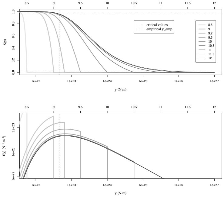
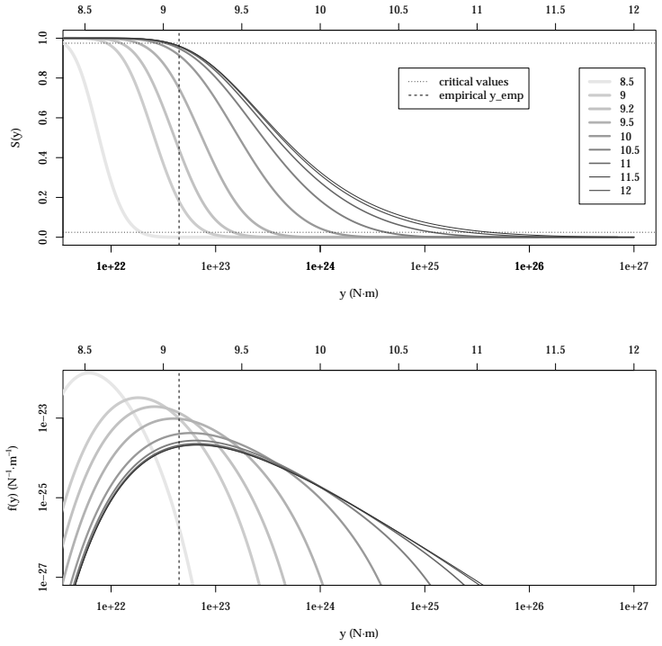
The load-bearing object is the maximum-order-statistic identity Fmax(y)=Prob[Y <= y]=[F(y)]^N, the cumulative distribution of the largest of N independent seismic moments. For the truncated power-law model, the maximum Y is exactly the maximum-likelihood estimator of the truncation parameter, so inverting Fmax(yp)=p gives 95% probability intervals for the estimated corner. For the tapered and truncated-gamma models the same percentile inversion is performed through closed forms involving implicit functions (the Lambert W function for the tapered model and the inverse incomplete gamma for the truncated gamma), and the empirical maximum is compared with those intervals to decide which corner values are compatible with the data. The machinery also supplies the sample size N needed to shrink an interval to a chosen width by solving the width equation; this replaces the earlier 'well-sampledness' criterion, which the paper shows is not a valid statistical test because it treats the observed maximum as fixed while N grows.
What would settle it
Recompute the Table 1 ranges after removing aftershocks from the global CMT catalog; if declustering moves the 95% intervals by more than a few tenths of a magnitude or pushes the empirical maximum outside them, the independence assumption is the weak link. The long-run check is to record the actual maximum to 2097 and see which of the 9.1, 9.3, or 9.5 branches of Table 1 it selects.
Extended reading notes
Core claim
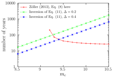
Contrary to an earlier analysis of the same catalog that concluded reliable estimation of the tapered corner magnitude would require about 200,000 years, the authors show that the correct use of the largest observed earthquake gives a much shorter horizon. The distribution of the maximum of N independent events is Fmax(y)=[F(y)]^N, so the observed largest magnitude can be tested against percentile intervals for each candidate model and each value of the corner magnitude. Inverting those percentiles yields, for each hypothetical true corner, the number N (or calendar year) at which the 95% interval narrows to a chosen width. Applying this to the 7,585 CMT events since 1977 leaves the corner magnitude unbounded above for all three models at the original catalog length, but already gives finite ranges by 2017, and under the paper's stated assumptions the projected 2097 ranges are much narrower: for the tapered model they are between about 0.5 and 1.0 magnitude wide, and for the truncated gamma between 0.5 and 1.4. The paper's Table 1 gives the predicted ranges for 2047 and 2097 conditional on the maximum magnitude observed in the interval (9.1, 9.3, or 9.5), showing that the outcome depends strongly on whether an event of magnitude 9.3 or larger occurs.
Load-bearing premise
The projected time windows assume the 7,585 catalogued earthquake magnitudes are independent, so the chance that the largest observed event stays below a value is the Nth power of the single-event chance; global catalogs contain aftershock clustering, and the paper states but does not test this dependence assumption.
Editorial extensions
If this is right
- By the end of 2017 the CMT data already give finite 95% ranges for the corner magnitude of the tapered (8.6-10.2), truncated power law (9.1-10.8), and truncated gamma (8.8-11.2) models, whereas the same data at mid-2012 allowed no upper bound.
- If no earthquake larger than magnitude 9.1 occurs before 2047, the truncated power law narrows the corner to 9.1-9.5; if a 9.3 event occurs instead, the tapered model allows 8.8-9.95, so the observation of a very large event is the main information carrier.
- The earlier conclusion that hundreds of thousands of years are needed for the tapered model is reversed; under the paper's assumptions, the 2097 ranges are narrow enough to distinguish among competing hypotheses about the tail.
- Seismic hazard should be evaluated by mixing tail models over the range of compatible corner values (Eq. 12) rather than by relying on a point estimate or on asymptotic standard errors, which the paper argues misdescribe the uncertainty.
Reading between the lines
- If aftershock clustering is strong enough to reduce the effective number of independent events below 7,585, the predicted narrowing dates would shift later than 2047 or 2097; this is testable because declustered catalogs would give wider percentile intervals.
- The same maximum-based percentile logic transfers to any heavy-tailed record where the scale parameter is debated and only a handful of extremes exist, such as storm surges, floods, or geomagnetic disturbances, provided a candidate tail family is specified.
- The calendar projections assume a constant global rate of 213.7 events per year and a fixed beta; a persistent rate change would move the dates but would not change the N-based widths, so the method is more robust than the specific years printed in Table 1.
- The mixture over corner values in Eq. (12) is equivalent to a Bayesian posterior under a 1/M_c prior; making that prior explicit would let hazard calculators report full predictive distributions instead of range endpoints.
Signed reviews
Editorial analysis
A structured set of objections, weighed in public.
Referee Report
Summary. The paper revisits the question of how much additional earthquake recording is needed to constrain the corner value (Mc or mc) of the global seismic-moment distribution. Using the global CMT catalog (7,585 events with magnitude ≥5.75, 1977–2012.5, extended to 2017) and fixing β=0.67, the authors compute 95% probability intervals for the maximum of N independent observations under three models — truncated power law (TPL), tapered GR (Tap), and truncated gamma (TrG) — via Fmax(y)=[F(y)]^N. From this they derive currently compatible ranges of mc (e.g., 8.6–10.2 for Tap) and conditional future ranges for hypothetical maxima in 2047 and 2097, and they argue that these ranges will shrink substantially by 2097, contrary to earlier claims that hundreds of thousands of years would be needed. They also show that the 'well-sampledness' criterion used by Zöller (2013) is statistically flawed.
Significance. The paper makes a useful methodological correction: the earlier 'well-sampledness' criterion (Zöller 2013) is replaced by a proper extremal significance test based on the distribution of the maximum, and the forward calculation is not circular because mc is not fitted to the observed maximum. The central probability calculation under the stated independence assumption is standard and appears correct, and the resulting Table 1 gives concrete, falsifiable conditional predictions. However, the headline claim that the range 'will' shrink by 2097 is not established by the conditional analysis.
major comments (3)
- [Abstract/Conclusions; Table 1 in 'Proper constraining of the corner seismic-moment: Tap and TrG cases'] The abstract and Conclusions assert that 'under reasonable assumptions, the range will be substantially reduced by the end of this century,' but Table 1 only lists compatible mc ranges conditional on hypothetical future maxima of 9.1, 9.3, and 9.5; no probabilities are assigned to these maxima. This is load-bearing, because models still compatible with current data can produce a future maximum that breaks the claimed reduction. For instance, the Tap model with mc=10.2 (the upper end of the 2017 compatible range) has S(10)≈3.2×10^-5, giving an expected 0.83 events of magnitude ≥10 in 120 years and a probability >50% of at least one; under a 10.0 maximum, the Tap compatible range shifts to roughly mc≈9.7–∞, so the range is not substantially reduced. The unconditional claim therefore needs either to be weakened to a conditional one or derived by integrating over the Poisson-distributed future maximum using a prior over mc.
- [Eq. (5); 'Proper constraining of the corner seismic-moment: TPL case'] Eq. (5) and all subsequent percentile calculations assume the 7,585 events are independent. The paper acknowledges this once ('assuming ... there is no dependence between the magnitudes') but does not quantify the effect of aftershock clustering on the 2047/2097 ranges. Since N enters Eqs. (10)–(11) and Table 1 through p^{1/N}, a modest reduction in the effective number of independent events can materially widen the reported intervals; a sensitivity analysis (e.g., using a declustered catalog or an effective N) is needed before the projections can be considered robust.
- [Throughout; Figs. 2–3 and Table 1] All entries use β=0.67, stated to be 'very close to the maximum-likelihood solution,' but no uncertainty in β is propagated. The compatible ranges of mc are monotone in β through the percentile formulas (10)–(11), so an error of, say, 0.05 in β could shift the bounds by several tenths of a magnitude. The paper needs at least a sensitivity analysis for β or a justification for treating it as known.
minor comments (5)
- [Discussion, Eq. (12)] Eq. (12) writes Stpl(x|Mc) in the integrand while the surrounding text is about the tapered model; this should be Stap (or a generic S_model).
- [Discussion, first sentence] The word 'assessment' is misspelled as 'assesment'.
- [Figure 3 caption] The caption uses the notation 'mpm' and '(mp, mp+0.95)' without defining which interval is symmetric and which is of minimum width; a brief explanation would improve readability.
- [SI captions, Figs. S4–S6] The captions misspell 'corresponding' as 'corresponing'.
- [Section 'Proper constraining of the corner seismic-moment: TPL case', last paragraph] The sentence 'we need to wait about 30 years to chose between these three answers' contains a typo: 'to chose' should be 'to choose'.
Circularity Check
Forward calculation, not circular: future corner-value ranges are conditional prediction-interval inversions, and the abstract's overstatement is a robustness issue, not a derivation that reduces to its inputs.
full rationale
The paper's core derivation is a forward calculation: from Eq. (5), Fmax(y)=[F(y)]^N, and the three model CDFs (Eqs. 2-4), it constructs 95% intervals for the maximum of N independent draws, then inverts the condition that a specified observed or hypothetical maximum lies inside that interval to obtain the compatible mc range shown in Table 1. This is a standard prediction-interval inversion, not a fit of mc to the data renamed as a prediction; the future maxima 9.1, 9.3, and 9.5 are explicitly hypothetical scenarios, as the paper says: 'This table also explores the values of these ranges in the future, depending on the hypothetical value of the maximum magnitude observed.' The abstract's unqualified wording that the range 'will be substantially reduced' is stronger than the conditional table, and the independence assumption behind Eq. (5) is acknowledged only in passing ('assuming that the TPL were the right model, that there is no dependence between the magnitudes, and that the long-term global earthquake rate and β were constant'). Those are correctness or robustness concerns, not circularity: the derivation does not assume what it sets out to show. The only numerical input plausibly taken from earlier same-author work is β=0.67, which is presented as a fixed value ('with β fixed to 0.67') and whose exact choice affects the numbers but not the logic; the self-citation to [20] is used to contrast previously computed standard errors, not to justify the present conclusion. No step in the derivation is equivalent by construction to its inputs, so no circular step can be exhibited.
Assumptions & free parameters
free parameters (3)
- β (power-law exponent minus 1) =
0.67
- Ra (annual rate above threshold) =
213.7 events per year
- a (lower cut-off seismic moment) =
5.31 x 10^17 N·m (moment magnitude 5.75)
assumptions (4)
- domain assumption The true global seismic-moment distribution belongs to one of the three families TPL, Tap, or TrG, with a single corner parameter Mc.
- domain assumption The N observations are independent, so the maximum has CDF Fmax(y)=[F(y)]^N.
- domain assumption The annual rate of events above the threshold is constant at 213.7 events per year.
- domain assumption The lower cut-off a and the shape parameter β are known without error.
Cite this review
Pith. "Pith review of Time window to constrain the corner value of the global seismic-moment distribution." pith.science (2026). https://pith.science/paper/6XGX5NKS
@misc{pith2026190802516,
  author       = {Pith},
  title        = {Pith review of: Time window to constrain the corner value of the global seismic-moment distribution},
  year         = {2026},
  howpublished = {\url{https://pith.science/paper/6XGX5NKS}},
  note         = {Machine review of arXiv:1908.02516}
}
read the original abstract
It is well accepted that, at the global scale, the Gutenberg-Richter (GR) law describing the distribution of earthquake magnitude or seismic moment has to be modified at the tail to properly account for the most extreme events. It is debated, though, how much additional time of earthquake recording will be necessary to properly constrain this tail. Using the global CMT catalog, we study how three modifications of the GR law that incorporate a corner-value parameter are compatible with the size of the largest observed earthquake in a given time window. Current data lead to a rather large range of parameter values (e.g., corner magnitude from 8.6 to 10.2 for the so-called tapered GR distribution). Updating this estimation in the future will strongly depend on the maximum magnitude observed, but, under reasonable assumptions, the range will be substantially reduced by the end of this century, contrary to claims in previous literature.
Figures


Figures from the paper (6 more)



Reference graph
Works this paper leans on
-
[1]
Why is Probabilistic Seismic Hazard Analysis (PSHA) still used? Phys Earth Planet Int
Mulargia F, Stark PB, Geller RJ. Why is Probabilistic Seismic Hazard Analysis (PSHA) still used? Phys Earth Planet Int. 2017;264:63–75
work page 2017
-
[2]
Utsu T. Representation and analysis of earthquake size distribution: a historical review and some new approaches. Pure Appl Geophys. 1999;155:509–535
work page 1999
-
[3]
Earthquakes: Models, Statistics, Testable Forecasts
Kagan YY. Earthquakes: Models, Statistics, Testable Forecasts. Wiley; 2014
work page 2014
-
[4]
Ben-Zion Y. Collective behavior of earthquakes and faults: continuum-discrete transitions, progressive evolutionary changes, and different dynamic regimes. Rev Geophys. 2008;46:RG4006
work page 2008
-
[5]
The energy release in great earthquakes
Kanamori H. The energy release in great earthquakes. J Geophys Res. 1977;82(20):2981–2987
work page 1977
-
[6]
Kanamori H, Brodsky EE. The physics of earthquakes. Rep Prog Phys. 2004;67:1429–1496
work page 2004
-
[7]
Criticality and self-organization in branching processes: application to natural hazards
Corral A, Font-Clos F. Criticality and self-organization in branching processes: application to natural hazards. In: Aschwanden M, editor. Self-Organized Criticality Systems. Open Academic Press, Berlin; 2013. p. 183–228. August 8, 2019 10/24
work page 2013
-
[8]
Scaling in the Timing of Extreme Events
Corral A. Scaling in the Timing of Extreme Events. Chaos Solit Fract. 2015;74:99–112
work page 2015
Show all 33 references
-
[9]
Seismic moment distribution revisited: I
Kagan YY. Seismic moment distribution revisited: I. Statistical results. Geophys J Int. 2002;148:520–541
2002
-
[10]
Universality of the Seismic Moment-frequency Relation
Kagan YY. Universality of the Seismic Moment-frequency Relation. Pure Appl Geophys. 1999;155:537–573
1999
-
[11]
Is the seismic moment-frequency relation universal? Geophys J Int
Godano C, Pingue F. Is the seismic moment-frequency relation universal? Geophys J Int. 2000;142:193–198
2000
-
[12]
Effect of the Sumatran mega-earthquake on the global magnitude cut-off and event rate
Main IG, Li L, McCloskey J, Naylor M. Effect of the Sumatran mega-earthquake on the global magnitude cut-off and event rate. Nature Geosci. 2008;1:142
2008
-
[13]
Earthquake size distribution: Power-law with exponent β≡ 1/2? Tectonophys
Kagan YY. Earthquake size distribution: Power-law with exponent β≡ 1/2? Tectonophys. 2010;490:103–114
2010
-
[14]
Convergence of the frequency-size distribution of global earthquakes
Bell AF, Naylor M, Main IG. Convergence of the frequency-size distribution of global earthquakes. Geophys Res Lett. 2013;40:2585–2589
2013
-
[15]
Fitting and goodness-of-fit test of non-truncated and truncated power-law distributions
Deluca A, Corral A. Fitting and goodness-of-fit test of non-truncated and truncated power-law distributions. Acta Geophys. 2013;61:1351–1394
2013
-
[16]
Convergence of the frequency-magnitude distribution of global earthquakes: Maybe in 200 years
Z¨ oller G. Convergence of the frequency-magnitude distribution of global earthquakes: Maybe in 200 years. Geophys Res Lett. 2013;40:3873–3877
2013
-
[17]
Undersampling power-law size distributions: effect on the assessment of extreme natural hazards
Geist EL, Parsons T. Undersampling power-law size distributions: effect on the assessment of extreme natural hazards. Nat Hazards. 2014;72:565–595
2014
-
[18]
Kluwer, Dordrecht; 2003
Mulargia F, Geller RJ, Earthquake Science and Seismic Risk Reduction. Kluwer, Dordrecht; 2003
2003
-
[19]
Remarks on the accelerated moment release model: problems of model formulation, simulation and estimation
Vere-Jones D, Robinson R, Yang W. Remarks on the accelerated moment release model: problems of model formulation, simulation and estimation. Geophys J Int. 2001;144(3):517–531
2001
-
[20]
Deviation from power law of the global seismic moment distribution
Serra I, Corral A. Deviation from power law of the global seismic moment distribution. Sci Rep. 2017;7:40045
2017
-
[21]
A modified form of the Gutenberg-Richter magnitude-frequency relation
Lomnitz-Adler J, Lomnitz C. A modified form of the Gutenberg-Richter magnitude-frequency relation. Bull Seismol Soc Am. 1979; 69(4) 1209–1214
1979
-
[22]
A First Course in Probability
Ross SM. A First Course in Probability. 8th ed. Prentice Hall, Englewood Cliffs; 2010
2010
-
[23]
Faster solutions of the inverse pairwise Ising problem
Broderick T, Dud´ ık M, Tkacik G, Schapireb RE, Bialek W. Faster solutions of the inverse pairwise Ising problem. arXiv. 2007;0712.2437
2007 arXiv
-
[24]
An Introduction to Statistical Modeling of Extreme Values
Coles S. An Introduction to Statistical Modeling of Extreme Values. Springer, London; 2001
2001
-
[25]
The global CMT project 2004-2010: Centroid-moment tensors for 13,017 earthquakes
Ekstr¨ om G, Nettles M, Dziewo´ nski AM. The global CMT project 2004-2010: Centroid-moment tensors for 13,017 earthquakes. Phys Earth Planet Int. 2012;200-201:1–9
2004
-
[26]
Determination of earthquake source parameters from waveform data for studies of global and regional seismicity
Dziewonski AM, Chou TA, Woodhouse JH. Determination of earthquake source parameters from waveform data for studies of global and regional seismicity. J Geophys Res. 1981;86:2825–2852. August 8, 2019 11/24
1981
-
[27]
Multiple CMT source analysis of the 2004 Sumatra earthquake
Tsai VC, Nettles M, Ekstr¨ om G, Dziewonski AM. Multiple CMT source analysis of the 2004 Sumatra earthquake. Geophys Res Lett. 2005;32(17):L17304
2004
-
[28]
Long-Term Perspectives on Giant Earthquakes and Tsunamis at Subduction Zones
Satake K, Atwater BF. Long-Term Perspectives on Giant Earthquakes and Tsunamis at Subduction Zones. Ann Rev Earth Planet Sci. 2007;35(1):349–374
2007
-
[29]
On the Lambert W function
Corless RM, Gonnet GH, Hare DEG, Jeffrey DJ, Knuth DE. On the Lambert W function. Adv Comp Math. 1996;5(1):329–359
1996
-
[30]
Phys Rev Lett
Corral A, Long-term clustering, scaling, and universality in the temporal occurrence of earthquakes. Phys Rev Lett. 2004; 92:108501
2004
-
[31]
Statistical Features of Earthquake Temporal Occurrence
Corral A. Statistical Features of Earthquake Temporal Occurrence. In: Bhattacharyya P, Chakrabarti BK, editors. Modelling Critical and Catastrophic Phenomena in Geoscience. Lecture Notes in Physics, 705. Springer, Berlin; 2007. p 191–221
2007
-
[32]
Time window to constrain the corner value of the global seismic-moment distribution
Mori˜ na D, Serra I, Puig P, Corral A. Probability estimation of a Carrington-like geomagnetic storm. Sci Rep. 2019; 9:2393. 1 Supporting information S1 Fig. ccdf S(x) and pdf f(x) of TPL distribution with β = 0.67, a corresponding to moment magnitude 5.75, and Mc correspondin...
2013
-
[33]
We provide graphical description of the three models for seismic-moment distributions in the paper as well as for the maximum of 7,585 of such events
Figures S1 to S6 Introduction. We provide graphical description of the three models for seismic-moment distributions in the paper as well as for the maximum of 7,585 of such events. We provide also the mathematical expressions for the probability density functions (pdf) of the...
2019
Reviewed August 14, 2026 · model on record in the stance chip above.
Discussion (0). Continue with ORCID to comment.