REVIEW 3 major objections 5 minor 69 references
Non-classicality at equilibrium and efficient predictions under non-commuting charges
T0 review · 3 major / 5 minor · reviewed 2026-08-06 · deepseek-v4-flash
Pith's one-line read For systems with non-commuting charges, the equilibrium distribution of a coarse observable is a generalized Gibbs law written in terms of weak values of energy and charge.
desk verdict Solid extension of observable statistical mechanics to non-commuting charges, but the headline 'efficient prediction' currently rests on an in-sample consistency check, not the advertised linear ansatz end-to-end. read the letter →
The pith
A machine-rendered reading of the paper's core claim, the machinery that carries it, and where it could break.
The reading
What carries the argument
The machinery is the generalized Gibbs-type equilibrium formula of Eq. (14), built from weak values defined by $O_w(\rho,A_j) = \mathrm{Tr}(\rho O A_j)/\mathrm{Tr}(\rho A_j)$. Its real parts, $\varepsilon_j = \mathrm{Re}[E_w(\rho,A_j)]$ and $q^a_j = \mathrm{Re}[Q^a_w(\rho,A_j)]$, act as effective outcome-resolved energy and charge entering a maximum-entropy weight; the imaginary parts must satisfy the first Equilibrium Equation via the chemical potentials. The derivation relies on a degeneracy theorem (Appendix A3) that makes the fine-grained outcome probabilities uniform within each highly degenerate eigenspace, on a small-mutual-information argument that justifies using only first moments of $H$ and $Q^a$ as constraints, and on Theorem I.1 linking degeneracy to non-Abelian symmetry.
What would settle it
Compute the classical mutual information $I_{\mathrm{eq}}(A,H)$ and $I_{\mathrm{eq}}(A,Q^a)$ for a specific coarse observable in an SU(2)-symmetric spin chain, pick an initial state or observable where these are not much smaller than the corresponding Shannon entropies, and check whether the total variation distance between Eq. (14) and the time-averaged distribution stays below 1%; a clear violation would refute the generality of the prediction.
Extended reading notes
Core claim
The central claim is that observable-level equilibrium in the presence of non-commuting charges is governed by the constrained maximum of the observable's Shannon entropy, and that the resulting distribution is characterized by weak values: $p^{\mathrm{est}}_j = d_j e^{-\beta_A \mathrm{Re}[E_w(\rho,A_j)] - \sum_a \mu_a \mathrm{Re}[Q^a_w(\rho,A_j)]}/Z_A$, where $\mathrm{Re}[E_w]$ and $\mathrm{Re}[Q^a_w]$ are the real parts of weak values of the Hamiltonian and of each conserved charge postselected on outcome $j$. The paper derives this from the first and second Equilibrium Equations, uses a degeneracy theorem to justify reducing the fine-grained distribution to the coarse one, and numerically confirms the formula for $N = 12, 14, 16$ with errors under 1% in total variation distance. It also proves a structural equivalence: a Hamiltonian is degenerate if and only if its symmetry group is non-Abelian, which links degeneracy directly to non-commuting charges. Finally, because the charges do not commute with the equilibrium state, the imaginary parts of their weak values can be nonzero at equilibrium; the paper shows this happens in about 20% of the explored SU(2)-breaking initial-state cases, witnessing Kirkwood-Dirac non-classicality without violating the Equilibrium Equations.
Load-bearing premise
The load-bearing premise is that a coarse observable shares so little mutual information with the energy and charges that maximizing entropy with only the first moments of H and Qa yields the right equilibrium distribution; if that smallness fails for some observable, Eq. (14) would need extra constraints and the prediction would break down.
Editorial extensions
If this is right
- For any sufficiently degenerate observable, the equilibrium distribution is computable from weak values of H and the charges, without energy eigenvectors or eigenvalues.
- Because degeneracy and non-commuting charges are equivalent, relaxation effects blamed on degeneracy cannot be separated from non-Abelian symmetry effects.
- Nonzero imaginary parts of charge weak values at equilibrium certify that the equilibrium description cannot be captured by a non-contextual classical model, even while the first Equilibrium Equation holds.
- For the spin model studied, the method improves on the non-Abelian thermal state precisely where coupling is not weak, which is also where the NATS derivation is not justified.
- The numerical agreement improves with system size from N = 12 to N = 16, suggesting the estimate becomes increasingly accurate in the thermodynamic limit.
Reading between the lines
- One could test Eq. (14) on a model with an SU(3) or larger non-Abelian symmetry: the paper predicts anomalies in imaginary weak values should appear for appropriate symmetry-breaking initial states, while the real parts may eventually become anomalous too.
- If the small-mutual-information condition is the true validity boundary, then deliberately constructing an observable that is finely correlated with an energy window or a charge sector should make Eq. (14) fail by an amount proportional to that mutual information; this would give a quantitative falsifier.
- The linear ansatz connecting $\varepsilon_j$ and $q^a_j$ to first moments of $H$ and $Q^a$ is empirical; an analytical derivation would turn the method into a parameter-free predictive scheme, but until then the method needs a few calibration points, so its practical status is interpolation rather than prediction from first principles.
Editorial analysis
A structured set of objections, weighed in public.
Referee Report
Summary. The paper generalizes Observable Statistical Mechanics to Hamiltonians with non-commuting conserved charges. It derives first and second equilibrium equations from a maximum-entropy principle, expresses the solution as a Gibbs-like distribution (Eq. 14) whose effective 'energy levels' and 'charge levels' are the real parts of weak values of H and the charges, and shows that these weak values can be anomalous (non-classical) at equilibrium. It also proves an equivalence between Hamiltonian degeneracy and the presence of a non-Abelian symmetry group (Theorem I.1). Numerical simulations on a non-integrable SU(2)-symmetric spin chain are used to verify the equilibrium equations and to compare the resulting distribution with the non-Abelian thermal state.
Significance. If the framework is correct, it provides a novel structural characterization of equilibrium distributions of coarse observables under non-commuting charges, connects equilibrium physics to weak values and Kirkwood-Dirac quasiprobabilities, and offers a potential route to predictions that avoid full diagonalization of the Hamiltonian. The derivation in Appendix A4 is careful and explicit, Theorem I.1 is clean and correctly proved for both finite and infinite dimensions, and the numerical checks of the First and Second Equilibrium Equations are extensive and supportive. The main weakness is that the 'efficient predictions' advertised in the title and abstract are not tested end-to-end: the numerical validation of Eq. (14) uses quantities extracted from the very equilibrium data being predicted, and the empirical linear ansatz (Eqs. 29-30) that is supposed to make the scheme predictive is validated only for the weak-value real parts, not for the resulting probability distributions.
major comments (3)
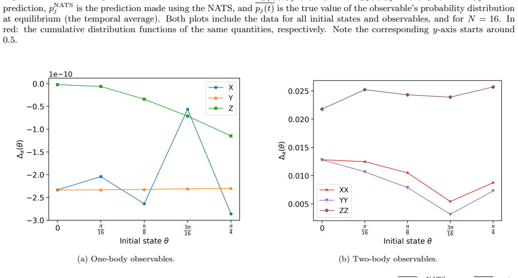
- [Sec. IV.D and Fig. 3] The numerical verification of Eq. (14) is in-sample. The text states that to compute pest_j the authors 'first obtain εj ≈ Rj(t)/pj(t) and qa_j ≈ Ra_j(t)/pj(t)' from the time-averaged evolution, and then fix β_A and μ_a by fitting or optimization on the same data. Thus Fig. 3 shows that the equilibrium distribution is consistent with a Gibbs form whose level parameters are read off from that very distribution; it does not demonstrate prediction of equilibrium without knowledge of the energy eigenvalues and eigenvectors. The genuinely predictive route, Eqs. (29)-(30), is never propagated to the probability distributions, and no total-variation distance is reported for the end-to-end scheme. I request an out-of-sample test: estimate εj and qa_j via Eqs. (29)-(30) for held-out initial states or observables, compute pest_j, and report the TVD against the time-averaged pj(t).
- [Sec. IV.C, Eqs. (29)-(30), and Fig. 2] The linear ansatz for εj and qa_j is explicitly admitted to be empirical and to lack an analytical derivation. Fig. 2 validates the ansatz only for εj and qa_j, using two or three data points to fix the coefficients, and it does not quantify how errors in the ansatz propagate into the final probability distribution. Since the 'efficient prediction' claim rests on this ansatz, the paper should either supply a derivation or provide a more extensive out-of-sample validation that includes the resulting distributions, not just the intermediate weak-value estimates.
- [Sec. II.D and Appendix A2] The validity of Eq. (14) is conditional on small mutual information between the coarse observable and the energy and charges. The paper gives heuristic arguments for this condition, but it never directly verifies the condition in the numerical experiments. Given that this small-mutual-information assumption is load-bearing for the maximum-entropy step, I suggest computing Ieq(A,H) and Ieq(A,Qa) from the simulated data and reporting them alongside the equilibrium-equation checks. This would confirm that the studied observables actually lie in the regime where the few-constraint maximum-entropy treatment is justified.
minor comments (5)
- [Eqs. (9), (10), (16), (18)] The notation '!' before '=' is used nonstandardly, apparently to mean 'is set to zero' or 'should equal'. This is confusing, especially combined with the surrounding equations; please define the notation explicitly or replace it with standard equality/stationarity notation.
- [Sec. IV.D] The procedure for determining β_A and μ_a^A is described only vaguely as 'either analytically or via numerical optimization'. Please specify for each observable which method was used, and report the fitted parameter values or the optimization objective, so that the results are reproducible.
- [Fig. 2 inset] The inset legend states that the grey line 'in this case coinciding with the green and orange lines' is the average energy E(θ). This makes the plot hard to read; using distinct markers or colors for overlapping curves would improve clarity.
- [Sec. IV.A vs. Appendix A5] The charges are defined with a 1/N factor in the main text (Eq. (24)) and in parts of Appendix A5, but the NATS construction in Appendix A5 uses Qa = Σ_i σ_i^a without the 1/N factor. Please flag this rescaling explicitly when moving between the two conventions, as it affects the magnitudes of qa and Δqa and could confuse readers.
- [Abstract and Sec. V] The abstract claims the framework can 'accurately estimate the equilibrium distribution of coarse observables without access to the energy eigenvalues and eigenvectors'. As argued in Major Comment 1, the numerical support for this specific claim is currently missing. Please either temper the claim to what is demonstrated or add the missing end-to-end test.
Circularity Check
Main numerical validation of Eq. (14) is in-sample: εj and qa_j are extracted from the same equilibrium distribution being predicted, and β, μ are fitted; the parameter-light linear-ansatz route is never tested end-to-end.
-
fitted input called prediction
[Section IV.D (Predicting the equilibrium distribution), around Eq. (14) and Fig. 3; see also Eqs. (15) and (20).]
"To compute our estimate pest_j ∝ e^{−βA εj − Σ_a μ_a qa_j}, we first obtain εj ≈ Rj(t)/pj(t) and qa_j ≈ Ra_j(t)/pj(t). Then, we calculate βA and the {μa_A}a either analytically or via numerical optimization. We quantify the closeness with pj(t) using the total variation distance."
By Eqs. (15) and (20), εj and qa_j are defined as Rj/pj and Ra_j/pj for the equilibrium state. The numerical recipe computes them from exactly the same time-averaged pj(t) that the estimate is later compared with, and βA, μa are fitted on the same data. The reported TVD < 1% therefore checks internal consistency of the max-entropy equations, not an out-of-sample prediction. The genuinely parameter-light route, Eqs. (29)-(30), is validated only for εj and qa_j individually (Fig. 2), and the end-to-end TVD obtained by inserting those linear-ansatz estimates into Eq. (14) is never reported. Thus the headline 'efficient predictions without spectral information' rests on an in-sample refit plus an untested empirical ansatz.
full rationale
The core theoretical derivation of Eq. (14) is not circular: it follows from a Jaynes-type constrained entropy maximization (Sec. II.A-II.B) with the Lagrange-multiplier solution, and the connection to weak values (Eq. (20)) is a mathematical identity. Theorem I.1 is proved in the paper, and the Anza-Gogolin-Huber-type theorem used to coarse-grain pjs to pj is restated and proved in Appendix A3, so those are independent mathematical inputs. The self-citations to Ref. [25] for the heuristic 'only first moments suffice' and for the linear ansatz Eqs. (29)-(30) are explicitly described as empirical and lacking a proper analytical derivation, so they are not disguised as external theorems; this lowers the circularity weight. The significant circularity is in the numerical validation of the central predictive claim: Sec. IV.D computes εj and qa_j from the same equilibrium data it then predicts, and fits β and μ on that data. Consequently Fig. 3 demonstrates that the equilibrium distribution can be parametrized in the Gibbs-like form of Eq. (14) with coefficients read off from the distribution itself, not that the scheme predicts the distribution from readily available information. The out-of-sample linear fits of Eqs. (29)-(30) cover only εj and qa_j, and the paper does not report the total variation distance of the resulting distributions. This leaves the end-to-end 'efficient prediction' claim partially supported by construction rather than by an independent test, warranting a score of 6.
Assumptions & free parameters
free parameters (5)
- γj, ηj, χj (linear fit coefficients for εj) =
not stated (fit to 2-3 data points)
- γa_j, χa_j (linear fit coefficients for qa_j) =
not stated
- βA (effective inverse temperature) =
obtained analytically or via numerical optimization
- µa_A (effective chemical potentials) =
obtained analytically or via numerical optimization
- β, µa (NATS inverse temperature and chemical potentials) =
fit to data in Appendix A5
assumptions (6)
- domain assumption Maximum entropy principle: the equilibrium distribution of a coarse observable is the one maximizing Shannon entropy under normalization, mean energy, and mean charge constraints.
- domain assumption The classical mutual information between a coarse observable and the energy/charges is much smaller than the Shannon entropy bounds, so only first moments are needed as constraints.
- domain assumption The initial state has an approximate microcanonical subspace, with charge standard deviations Δqa scaling at most as √N.
- domain assumption The observables are coarse enough to satisfy dj(dj-1) ≥ nE+1, so the generalized Anza-Gogolin-Huber theorem applies.
- domain assumption The observable equilibrates in the time-average sense.
- standard math Spectral theorem and direct integral decomposition for the infinite-dimensional version of Theorem I.1.
Cite this review
Pith. "Pith review of Non-classicality at equilibrium and efficient predictions under non-commuting charges." pith.science (2026). https://pith.science/paper/745MVUTM
@misc{pith2026250722882,
  author       = {Pith},
  title        = {Pith review of: Non-classicality at equilibrium and efficient predictions under non-commuting charges},
  year         = {2026},
  howpublished = {\url{https://pith.science/paper/745MVUTM}},
  note         = {Machine review of arXiv:2507.22882}
}
read the original abstract
A quantum thermodynamic system can conserve non-commuting observables, but the consequences of this phenomenon on relaxation are still not fully understood. We investigate this problem by leveraging an observable-dependent approach to equilibration and thermalization in isolated quantum systems. We extend such approach to scenarios with non-commuting charges, and show that it can accurately estimate the equilibrium distribution of coarse observables without access to the energy eigenvalues and eigenvectors. Our predictions do not require weak coupling and are not restricted to local observables, thus providing an advantage over the non-Abelian thermal state. Within this approach, weak values and quasiprobability distributions emerge naturally and play a crucial role in characterizing the equilibrium distributions of observables. We show and numerically confirm that, due to charges' non-commutativity, these weak values can be anomalous even at equilibrium, which has been proven to be a proxy for non-classicality. Our work thus uncovers a novel connection between the relaxation of observables under non-commuting charges, weak values, and Kirkwood-Dirac quasiprobability distributions.
Figures


Figures from the paper (7 more)




Reference graph
Works this paper leans on
-
[1]
Huang, Statistical mechanics, 2nd ed
K. Huang, Statistical mechanics, 2nd ed. (Wiley, New York, 1987)
work page 1987
- [2]
-
[3]
E. Hinds Mingo, Y. Guryanova, P. Faist, and D. Jen- nings, in Thermodynamics in the Quantum Regime: Fundamental Aspects and New Directions, Fundamental Theories of Physics, edited by F. Binder, L. A. Correa, C. Gogolin, J. Anders, and G. Adesso (Springer Interna- tional Publishing, Cham, 2018) pp. 751–771
work page 2018
-
[4]
N. Yunger Halpern, P. Faist, J. Oppenheim, and A. Win- ter, Nature Communications 7, 12051 (2016), number: 1 Publisher: Nature Publishing Group
work page 2016
-
[5]
N. Y. Halpern, Journal of Physics A: Mathematical and Theoretical 51, 094001 (2018), publisher: IOP Publish- ing
2018
-
[6]
N. Yunger Halpern, M. E. Beverland, and A. Kalev, Physical Review E 101, 042117 (2020), publisher: Amer- ican Physical Society
work page 2020
- [7]
-
[8]
J. D. Noh, Physical Review E 107, 014130 (2023), pub- lisher: American Physical Society
work page 2023
Show all 69 references
-
[9]
Popescu, A
S. Popescu, A. B. Sainz, A. J. Short, and A. Win- ter, Philosophical Transactions of the Royal Society A: Mathematical, Physical and Engineering Sciences 376, 20180111 (2018), publisher: Royal Society
2018
-
[10]
Popescu, A
S. Popescu, A. B. Sainz, A. J. Short, and A. Winter, Physical Review Letters 125, 090601 (2020), publisher: American Physical Society
2020
-
[11]
Z. B. Khanian, M. N. Bera, A. Riera, M. Lewenstein, and A. Winter, Annales Henri Poincar´ e24, 1725 (2023)
2023
-
[12]
Lostaglio, D
M. Lostaglio, D. Jennings, and T. Rudolph, New Journal of Physics 19, 043008 (2017), publisher: IOP Publishing
2017
-
[13]
Guryanova, S
Y. Guryanova, S. Popescu, A. J. Short, R. Silva, and P. Skrzypczyk, Nature Communications 7, 12049 (2016), number: 1 Publisher: Nature Publishing Group
2016
-
[14]
Reimann, Physical Review Letters 101, 190403 (2008), publisher: American Physical Society
P. Reimann, Physical Review Letters 101, 190403 (2008), publisher: American Physical Society
2008
-
[15]
Murthy, A
C. Murthy, A. Babakhani, F. Iniguez, M. Srednicki, and N. Yunger Halpern, Physical Review Letters 130, 140402 (2023), publisher: American Physical Society
2023
-
[16]
Lasek, J
A. Lasek, J. D. Noh, J. LeSchack, and N. Y. Halpern, Numerical evidence for the non-Abelian eigenstate ther- malization hypothesis (2024), arXiv:2412.07838 [quant- ph]
2024 arXiv
-
[17]
Patil and M
R. Patil and M. Rigol, Physical Review B 111, 205126 (2025), publisher: American Physical Society
2025
-
[18]
Manzano, J
G. Manzano, J. M. Parrondo, and G. T. Landi, PRX Quantum 3, 010304 (2022), publisher: American Physi- cal Society
2022
-
[19]
Shahidani, Physical Review A 105, 063516 (2022), publisher: American Physical Society
S. Shahidani, Physical Review A 105, 063516 (2022), publisher: American Physical Society
2022
-
[20]
Upadhyaya, W
T. Upadhyaya, W. F. Braasch, G. T. Landi, and N. Y. Halpern, PRX Quantum 5, 030355 (2024), publisher: American Physical Society
2024
-
[21]
Majidy, A
S. Majidy, A. Lasek, D. A. Huse, and N. Yunger Halpern, Physical Review B 107, 045102 (2023), publisher: Amer- ican Physical Society
2023
-
[22]
A. C. Potter and R. Vasseur, Physical Review B 94, 224206 (2016), publisher: American Physical Society
2016
-
[23]
I. V. Protopopov, W. W. Ho, and D. A. Abanin, Phys- ical Review B 96, 041122 (2017), publisher: American Physical Society
2017
-
[24]
Majidy, Nature Communications 15, 8246 (2024), pub- lisher: Nature Publishing Group
S. Majidy, Nature Communications 15, 8246 (2024), pub- lisher: Nature Publishing Group
2024
-
[25]
Scarpa, A
L. Scarpa, A. Alhajri, V. Vedral, and F. Anza, Ob- servable Statistical Mechanics (2025), arXiv:2309.15173 [quant-ph]. 12
2025 arXiv
-
[26]
Anz` a and V
F. Anz` a and V. Vedral, Scientific Reports 7, 44066 (2017), number: 1 Publisher: Nature Publishing Group
2017
-
[27]
F. Anza, C. Gogolin, and M. Huber, Physical Review Letters 120, 150603 (2018), publisher: American Physi- cal Society
2018
-
[28]
Anza, Pure states statistical mechanics: on its foundations and applications to quantum gravity , http://purl.org/dc/dcmitype/Text, University of Oxford (2018)
F. Anza, Pure states statistical mechanics: on its foundations and applications to quantum gravity , http://purl.org/dc/dcmitype/Text, University of Oxford (2018)
2018
-
[29]
E. T. Jaynes, Physical Review 108, 171 (1957), publisher: American Physical Society
1957
-
[30]
E. T. Jaynes, Physical Review 106, 620 (1957), publisher: American Physical Society
1957
-
[31]
E. T. Jaynes, in E. T. Jaynes: Papers on Probabil- ity, Statistics and Statistical Physics, Synthese Library, edited by R. D. Rosenkrantz (Springer Netherlands, Dor- drecht, 1989) pp. 39–76
1989
-
[32]
Gogolin and J
C. Gogolin and J. Eisert, Reports on Progress in Physics 79, 056001 (2016), publisher: IOP Publishing
2016
-
[33]
Goldstein, T
S. Goldstein, T. Hara, and H. Tasaki, Physical Review Letters 111, 140401 (2013), publisher: American Physi- cal Society
2013
-
[34]
A. S. L. Malabarba, L. P. Garc ´ ıa-Pintos, N. Linden, T. C. Farrelly, and A. J. Short, Physical Review E 90, 012121 (2014), publisher: American Physical Society
2014
-
[35]
Anza, Entropy 20, 744 (2018), number: 10 Publisher: Multidisciplinary Digital Publishing Institute
F. Anza, Entropy 20, 744 (2018), number: 10 Publisher: Multidisciplinary Digital Publishing Institute
2018
-
[36]
F. H. L. Essler and M. Fagotti, Journal of Statistical Me- chanics: Theory and Experiment 2016, 064002 (2016)
2016
-
[37]
Sutherland, Beautiful Models: 70 Years of Exactly Solved Quantum Many-Body Problems (WORLD SCI- ENTIFIC, 2004)
B. Sutherland, Beautiful Models: 70 Years of Exactly Solved Quantum Many-Body Problems (WORLD SCI- ENTIFIC, 2004)
2004
-
[38]
L. P. Garc ´ ıa-Pintos, N. Linden, A. S. Malabarba, A. J. Short, and A. Winter, Physical Review X 7, 031027 (2017), publisher: American Physical Society
2017
-
[39]
Yunger Halpern and S
N. Yunger Halpern and S. Majidy, npj Quantum Informa- tion 8, 1 (2022), number: 1 Publisher: Nature Publishing Group
2022
-
[40]
L. D. Landau, E. M. Lifshitz, and L. P. Pitaevskij, Statis- tical physics. Part 1, 3rd ed., Course of theoretical physics / L. D. Landau and E. M. Lifshitz No. 5 (Elsevier But- terworth Heinemann, Amsterdam Heidelberg, 2011)
2011
-
[41]
R. C. Tolman, The principles of statistical mechanics, unabridged and unaltered republ. of the original (1938) ed ed., Dover books on physics (Dover, New York, NY, 1980)
1938
-
[42]
Balian and N
R. Balian and N. L. Balazs, Annals of Physics 179, 97 (1987)
1987
-
[43]
T. M. Cover and J. A. Thomas, Elements of Information Theory, 1st ed. (Wiley, 2005)
2005
-
[44]
Aharonov, D
Y. Aharonov, D. Z. Albert, and L. Vaidman, Physical Review Letters 60, 1351 (1988)
1988
-
[45]
Dressel, M
J. Dressel, M. Malik, F. M. Miatto, A. N. Jordan, and R. W. Boyd, Reviews of Modern Physics 86, 307 (2014), publisher: American Physical Society
2014
-
[46]
Lostaglio, A
M. Lostaglio, A. Belenchia, A. Levy, S. Hern´ andez- G´ omez, N. Fabbri, and S. Gherardini, Quantum7, 1128 (2023), publisher: Verein zur F¨ orderung des Open Access Publizierens in den Quantenwissenschaften
2023
-
[47]
D. R. M. Arvidsson-Shukur, W. F. B. Jr, S. D. Bi` evre, J. Dressel, A. N. Jordan, C. Langrenez, M. Lostaglio, J. S. Lundeen, and N. Y. Halpern, New Journal of Physics 26, 121201 (2024), publisher: IOP Publishing
2024
-
[48]
Gammelmark, B
S. Gammelmark, B. Julsgaard, and K. Mølmer, Physical Review Letters 111, 160401 (2013), publisher: American Physical Society
2013
-
[49]
L. P. Garc ´ ıa-Pintos and J. Dressel, Physical Review A96, 062110 (2017), publisher: American Physical Society
2017
-
[50]
M. F. Pusey, Physical Review Letters 113, 200401 (2014), publisher: American Physical Society
2014
-
[51]
Kunjwal, M
R. Kunjwal, M. Lostaglio, and M. F. Pusey, Physical Re- view A 100, 042116 (2019), publisher: American Physi- cal Society
2019
-
[52]
Dressel, Physical Review A 91, 032116 (2015), pub- lisher: American Physical Society
J. Dressel, Physical Review A 91, 032116 (2015), pub- lisher: American Physical Society
2015
-
[53]
Haegeman, J
J. Haegeman, J. I. Cirac, T. J. Osborne, I. Piˇ zorn, H. Ver- schelde, and F. Verstraete, Physical Review Letters 107, 070601 (2011), publisher: American Physical Society
2011
-
[54]
Haegeman, C
J. Haegeman, C. Lubich, I. Oseledets, B. Vandereycken, and F. Verstraete, Physical Review B 94, 165116 (2016), publisher: American Physical Society
2016
-
[55]
Collura, G
M. Collura, G. Lami, N. Ranabhat, and A. San- tini, Tensor Network Techniques for Quantum Compu- tation (SISSA Medialab S.r.l., 2024) accepted: 2024-12- 19T11:03:53Z
2024
-
[56]
Lostaglio, Physical Review Letters 125, 230603 (2020), publisher: American Physical Society
M. Lostaglio, Physical Review Letters 125, 230603 (2020), publisher: American Physical Society
2020
-
[57]
Riera, C
A. Riera, C. Gogolin, and J. Eisert, Physical Review Let- ters 108, 080402 (2012), publisher: American Physical Society
2012
-
[58]
A. J. Short and T. C. Farrelly, New Journal of Physics 14, 013063 (2012), publisher: IOP Publishing
2012
-
[59]
B. C. Hall, Quantum Theory for Mathematicians, Gradu- ate Texts in Mathematics, Vol. 267 (Springer, New York, NY, 2013)
2013
-
[60]
Takesaki, ed., Theory of Operator Algebras I (Springer, New York, NY, 1979)
M. Takesaki, ed., Theory of Operator Algebras I (Springer, New York, NY, 1979)
1979
-
[61]
M. A. Nielsen and I. L. Chuang, Quantum Computation and Quantum Information: 10th Anniversary Edition (Cambridge University Press, 2010)
2010
-
[62]
Bengtsson and K
I. Bengtsson and K. Zyczkowski, Geometry of Quan- tum States: An Introduction to Quantum Entanglement (Cambridge University Press, Cambridge, 2006)
2006
-
[63]
K. F. Riley, M. P. Hobson, and S. J. Bence, Mathematical Methods for Physics and Engineering: A Comprehensive Guide, 3rd ed. (Cambridge University Press, 2006)
2006
-
[64]
L. E. Reichl, A Modern Course in Statistical Physics, 1st ed. (Wiley, 2016)
2016
-
[65]
Tasaki, Physical Review Letters 80, 1373 (1998), pub- lisher: American Physical Society
H. Tasaki, Physical Review Letters 80, 1373 (1998), pub- lisher: American Physical Society
1998
-
[66]
Reimann, New Journal of Physics 12, 055027 (2010)
P. Reimann, New Journal of Physics 12, 055027 (2010)
2010
-
[67]
A. S. Trushechkin, M. Merkli, J. D. Cresser, and J. An- ders, A VS Quantum Science4, 012301 (2022)
2022
-
[68]
position
H. Dong, S. Yang, X. F. Liu, and C. P. Sun, Physical Re- view A 76, 044104 (2007), publisher: American Physical Society. 13 APPENDIX These appendices are organized as follows. In Sec. A1, we prove the infinite-dimensional version of Theorem I.1. This completes our argument tha...
2007
-
[69]
on average
guarantees finding dj generalized Bloch vectors ⃗bjs that obey the conditions in Eqs. (A6) and (A7) by choosing them to be the facet vectors of such a simplex. We thus required2 j −2−M ≥ dj −1, equivalently dj(dj −1) ≥ M +1. Remark. If the projectors {Πn} are rank-1, i.e., dn ...
Reviewed August 6, 2026 · model on record in the stance chip above.
Discussion (0). Sign in to comment.