REVIEW 3 major objections 4 minor 55 references
Solar wind entry into Mercury's magnetosphere: Simulation results for the second swingby of BepiColombo
T0 review · 3 major / 4 minor · reviewed 2026-08-10 · deepseek-v4-flash
Pith's one-line read A global hybrid simulation of BepiColombo's second Mercury swingby finds solar wind protons entering the magnetosphere with energies from a few eV to about 10 keV, and maps the plasma regions crossed by the spacecraft.
desk verdict Useful trajectory-spectrum tool for Mercury hybrid simulations; fix the abstract's misplaced 10 keV and the qualitative/quantitative contradiction before publication. read the letter →
The pith
A machine-rendered reading of the paper's core claim, the machinery that carries it, and where it could break.
The reading
What carries the argument
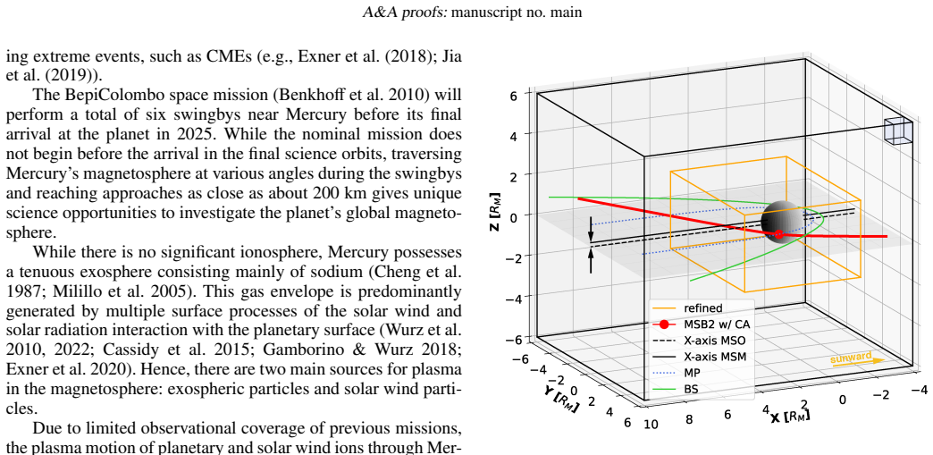
The central machinery is the AIKEF global hybrid simulation, in which protons are followed as kinetic particles and electrons act as a massless, charge-neutralizing fluid; magnetic reconnection is handled self-consistently through anomalous resistivity, and Mercury's surface absorbs impacting particles. The trajectory-analysis tool built on top is the second essential piece: at each point along the MSB2 path, all simulated protons within a sphere of radius 5 ion inertial lengths (about 200 km) are collected and binned into a 60-bin logarithmic energy histogram from 1 eV to 20 keV, giving an omnidirectional energy spectrum with more than 1000 particles per point. This extraction method connects the global simulation to the spacecraft's actual path and lets the authors identify magnetospheric regions from distinct particle populations in the spectrum.
What would settle it
Compare the model's predicted proton energy spectrum and boundary-crossing times along the MSB2 trajectory with BepiColombo's ion and magnetic field measurements from 23 June 2022; a mismatch in the times of the inbound or outbound magnetopause or bow shock crossings, or the absence of the predicted roughly 10 keV dawnside tail population, would show that the steady-state snapshot does not represent the actual flyby.
Extended reading notes
Core claim
Using the AIKEF global hybrid code, with ions treated kinetically and electrons as a massless fluid, the authors built a quasi-steady-state model of Mercury's magnetosphere from BepiColombo's outbound IMF measurements and MESSENGER-average solar wind parameters. They then extracted all simulated protons within about 200 km (5 solar-wind ion inertial lengths) of each point on the MSB2 trajectory and binned their velocities into an omnidirectional energy spectrum. The spectrum shows solar wind protons throughout the magnetosphere: a few eV near closest approach on the dawnside, roughly 50 eV in the tail lobes, 20 to 200 eV while grazing the tail current sheet, energies up to 10 keV near the dawnside flanks of the tilted current sheet, and about 4 keV in the pre-terminator dawnside magnetosheath. The authors use the spectrum together with density and current-density slices to assign boundary crossings along the flyby: inbound magnetopause, tail-current-sheet graze, outbound magnetopause, and outbound bow shock, plus a field-aligned ion beam in the foreshock. They conclude that solar wind entry is the main source of the ions and that the simulation reproduces the empirical stand-off distances, with the magnetopause at 1.45 RM and the bow shock at 1.85 RM at the subsolar point, while revealing a dawn-dusk asymmetry in magnetosheath thickness caused by the oblique IMF.
Load-bearing premise
The whole flyby comparison rests on treating one quasi-steady snapshot of the simulation as a stand-in for the actual one-to-two-hour encounter, even though Mercury's magnetosphere can reconfigure on a roughly two-minute timescale.
Editorial extensions
If this is right
- BepiColombo's particle instruments can be checked directly against the predicted spectrum; matching boundary crossings would validate the model and the inferred solar wind entry.
- The predicted 10 keV population near the dawnside tail current sheet gives a concrete signature of reconnection-accelerated solar wind protons that the spacecraft should have encountered after closest approach.
- The dawn-dusk asymmetry in bow shock and magnetosheath thickness implies that inbound and outbound crossings during MSB2 should exhibit different shock strengths and foreshock activity, which the magnetometer data can test.
- The same snapshot-extraction method can be replayed along the trajectories of the remaining BepiColombo swingbys to produce quick forecast spectra for operations and measurement planning.
- If the few-eV population near closest approach is real, it implies the solar wind supplies low-energy ions in the near-surface magnetosphere, a region the spacecraft sampled for the first time.
Reading between the lines
- Going beyond the paper, the same extraction method applied to a time series of snapshots would directly test whether the two-minute Dungey cycle blurs the predicted boundary times along a one-to-two-hour flyby.
- Going beyond the paper, the model's omission of planetary ions means the few-eV part of the spectrum is probably incomplete; including exospheric ions such as Na+ could change the closest-approach interpretation.
- Going beyond the paper, the dawn-dusk asymmetry should rotate with the IMF clock angle, so the same simulation setup could be run at different upstream conditions to produce a forecast library for the remaining swingbys.
- Going beyond the paper, confirmation of the foreshock ion beam in outbound data would make Mercury a natural small-scale laboratory for quasi-parallel shock acceleration.
Editorial analysis
A structured set of objections, weighed in public.
Referee Report
Summary. The paper uses the global 3D hybrid code AIKEF to simulate the interaction of the solar wind with Mercury's magnetosphere under conditions representative of BepiColombo's second Mercury swingby (MSB2). Upstream solar wind parameters are taken from MESSENGER average values, and the IMF direction is derived from Mio MGF measurements; no free parameters are fitted to the target results. The authors compute proton energy spectra along the MSB2 trajectory by extracting particles within a 5 ion-inertial-length cloud from a single quasi-steady simulation snapshot at 760 s. They report a dawn-dusk magnetosheath thickness asymmetry, magnetopause and bow shock stand-off distances of R_MP = 1.45 R_M and R_BS = 1.85 R_M, and solar wind protons penetrating into the magnetosphere with energies ranging from a few eV near closest approach to about 6-10 keV near the dawnside tail current sheet and about 4 keV in the dayside magnetosheath. They also identify boundary crossings and region-specific particle populations along the trajectory, and discuss implications for interpreting BepiColombo swingby data.
Significance. If the results are taken as a faithful representation of the MSB2 encounter, the paper provides a useful method for extracting trajectory-aligned ion energy spectra from hybrid simulations and gives concrete predictions for the plasma regions crossed during MSB2. The study is strengthened by the absence of fitted parameters: inputs come from independent measurements (MESSENGER averages, Mio MGF), and outputs are compared with empirical models from other authors. The spectrum-extraction approach is flexible and reusable for future swingbys. However, the significance is substantially qualified by the single-snapshot assumption; because the real flyby lasted 1-2 hours and Mercury's Dungey cycle is about 2 minutes, the trajectory-specific predictions are not yet verified as quantitative forecasts. The paper also contains internal inconsistencies between the abstract, the results section, and the conclusions about where the 10 keV population is located and about whether the results are qualitative or quantitative.
major comments (3)
- [Sections 2.1, 3.2, and 4] The single-snapshot assumption is load-bearing and is not adequately addressed. Section 2.1 states that the simulation is run for about 760 s to reach a quasi-steady state, and Section 3.2 explains that the spectrum in Fig. 3 is obtained by mapping the spatial positions of the MSB2 trajectory through this one quasi-stationary state. Section 4 then concedes that Mercury's Dungey cycle is about 2 min and that the ~1-2 h flyby 'might allow reconfigurations that potentially affect boundary positions and orientations.' Because the labeled crossings (1)-(5) in Fig. 3 and the energies assigned to each region (few eV in the magnetosphere, ~6-10 keV near the dawnside tail current sheet, ~4 keV in the dayside magnetosheath) are trajectory-specific, they are not guaranteed to represent what BepiColombo actually encountered during MSB2. The authors should either add a time-dependent treatment or explicitly demote all trajectory-specific timings and energy assignments to illustrative products of a single quasi-steady configuration.
- [Abstract and Section 3.2] The abstract's statement that energies reach 'up to 10 keV in the magnetosheath' contradicts the body of the paper. Section 3.2 locates the ~6-10 keV population 'near the (dawnside) flanks of the tilted tail current sheet' and states that the dayside magnetosheath energy ranges 'from 10 eV up to about 4 keV'; Section 4 likewise summarizes 'up to about 4 keV in the magnetosheath region on the pre-terminator dawnside.' The abstract must be corrected to match the body, or the body must be revised if the abstract was intended.
- [Sections 3.2 and 4] The paper gives contradictory epistemic status to its own results. Section 3.2 states that 'our simulation results are more appropriately viewed as a qualitative representation of the real flyby,' whereas Section 4 states that 'our results should be regarded as a quantitative representation, especially if compared to particle measurements during MSB2.' Since the abstract and conclusions promise quantitative estimates of boundary crossings and energies along the trajectory, this contradiction is central. The authors should choose one characterization, justify it, and adjust the title, abstract, and conclusions accordingly.
minor comments (4)
- [Section 3.2] The horizontal dashed line in Fig. 3 is called the 'solar wind initialization temperature of 1 keV,' but 1 keV is approximately the bulk kinetic energy of a 400 km/s proton, while Table 1 lists the ion temperature as 17 eV. Please use 'energy' rather than 'temperature' in this description.
- [Figure 3] The caption labels v_x < 0 as 'sunward'; since the MASO X-axis is anti-sunward this is correct, but the coordinate convention should be stated in the caption for readers not familiar with MASO.
- [Section 3.1] The phrase 'The lowest number densities of > 0.01 cm^-3' is ambiguous; a threshold or a range should be stated explicitly.
- [Throughout] There are several typographical issues, including 'magnetopshere' (Sections 2.1 and 4), 'di fference' (Section 3.1), and 'Insitute' (Acknowledgements); please proofread the manuscript.
Circularity Check
No significant circularity: simulation inputs are independent measurements and outputs are checked against external empirical models.
full rationale
The derivation chain is not circular. The AIKEF hybrid simulation is initialized with upstream parameters taken from independent observations (four years of MESSENGER averages for solar wind density, velocity, temperature, and IMF magnitude; Mio/MGF for the IMF direction during MSB2) and with a planetary field from Anderson et al. (2012). No parameter is fitted to the quantities the paper later presents as results: the stand-off distances R_MP = 1.45 R_M and R_BS = 1.85 R_M are compared with, not regressed to, the empirical Slavin/Winslow/Korth models, and the proton energy spectra are extracted from the simulation snapshot rather than matched to BepiColombo measurements. The only input-linked spectral feature is the peak near 1 keV, which the paper itself identifies as the solar wind input bulk energy ('The particle energy peaks are just under 1 keV, which equates to the solar wind input energy'); this is an upstream boundary condition, not a fitted parameter renamed as a prediction. The paper also explicitly flags its main validity limitation instead of hiding it: Section 4 states 'we utilized a steady state snapshot ... the dynamics of the system are not covered' and that the one-to-two hour flyby 'might allow reconfigurations that potentially affect boundary positions and orientations.' That caveat reduces confidence in trajectory-timed region identification but is not circularity. Self-citations to the AIKEF code (Muller et al. 2011) and to prior Mercury hybrid simulations (Exner et al. 2018, 2020) are normal method references and are not load-bearing in a way that forces the results. Internal inconsistencies, such as the abstract's 'up to 10 keV in the magnetosheath' versus Section 3.2 placing the 10 keV population near the dawnside tail current sheet and about 4 keV in the magnetosheath, are correctness issues rather than circularity.
Assumptions & free parameters
assumptions (5)
- domain assumption Upstream solar wind parameters from four years of MESSENGER averages (density 40 cm^-3, velocity 400 km/s, temperature 17 eV, IMF magnitude 24.2 nT) are representative of conditions during MSB2.
- domain assumption The IMF direction measured by Mio MGF during the outbound phase (components -0.79, 0.59, 0.06) is the relevant upstream IMF for the whole magnetosphere interaction.
- ad hoc to paper A single quasi-steady state snapshot after 760 s of simulation time represents the magnetosphere along the MSB2 trajectory over the one-to-two hour flyby.
- domain assumption Simulating only solar wind protons, with Mercury's surface as a perfect absorber and no exospheric ions, is sufficient to capture the entry and energy profile of solar wind particles.
- domain assumption Collecting particles within a constant radius of 5 solar-wind ion inertial lengths (~200 km) at each trajectory point yields an omnidirectional spectrum representative of what the spacecraft particles instruments would observe.
Cite this review
Pith. "Pith review of Solar wind entry into Mercury's magnetosphere: Simulation results for the second swingby of BepiColombo." pith.science (2026). https://pith.science/paper/7C6LLBIP
@misc{pith2026250105363,
  author       = {Pith},
  title        = {Pith review of: Solar wind entry into Mercury's magnetosphere: Simulation results for the second swingby of BepiColombo},
  year         = {2026},
  howpublished = {\url{https://pith.science/paper/7C6LLBIP}},
  note         = {Machine review of arXiv:2501.05363}
}
read the original abstract
Context. We use a global 3D hybrid plasma model to investigate the interaction between Mercury's magnetosphere and the solar wind for the second BepiColombo swingby, evaluate magnetospheric regions, and study the typical energy profile of protons. Aims. The objective of this study is to gain a better understanding of solar wind entry and analyze simulated plasma data along a trajectory using BepiColombo swingby 2 conditions, with the goal of enhancing our comprehension of measurement data and potentially providing forecasts for future swingbys. Methods. To model Mercury's plasma environment, we used the hybrid code AIKEF and developed a method to extract the particle (ion) data in order to compute the proton energy spectrum along the trajectory of BepiColombo during its second Mercury swingby on June 23, 2022. We evaluate magnetopause and bow shock stand-off distances under average upstream solar wind conditions with the Interplanetary Magnetic Field (IMF) condition derived from the BepiColombo magnetic field measurements during the second Mercury swingby. Results. We found that the magnetosheath on the quasi-perpendicular (dusk) side of the bow shock is thicker than that on the quasi-parallel (dawn) side, where a foreshock is formed. Multiple plasma populations can be extracted from our modeled energy spectra that assist in identifying magnetospheric regions. We observed protons of solar wind origin entering Mercury's magnetosphere. Their energies range from a few electron volts in the magnetosphere up to 10 keV in the magnetosheath.
Figures


Reference graph
Works this paper leans on
-
[1]
Aizawa, S., Griton, L. S., Fatemi, S., et al. 2021, Planetary and Space Science, 198, 105176, doi:10.1016/j.pss.2021.105176
-
[2]
Bobrovnikov, S., Slavin, J., & Saran- tos, M
Alexeev, I., Belenkaya, E., Yu. Bobrovnikov, S., Slavin, J., & Saran- tos, M. 2008, Journal of Geophysical Research: Space Physics, 113, doi:10.1029/2008JA013368
-
[3]
Anderson, B. J., Acuña, M. H., Korth, H., et al. 2008, Science, 321, 82, doi:10.1126/science.1159081
-
[4]
Anderson, B. J., Johnson, C. L., Korth, H., et al. 2012, Journal of Geophysical Research: Planets, 117, doi:10.1029/2012JE004159
-
[5]
N., Poh, G., Odstrcil, D., et al
Baker, D. N., Poh, G., Odstrcil, D., et al. 2013, Journal of Geophysical Research: Space Physics, 118, 45, doi:10.1029/2012JA018064
-
[6]
Baker, D. N., Pulkkinen, T. I., Angelopoulos, V ., Baumjohann, W., & McPher- ron, R. L. 1996, J. Geophys. Res., 101, 12975, doi:10.1029/95JA03753
-
[7]
Baumjohann, W., Matsuoka, A., Narita, Y ., et al. 2020, Space Sci. Rev., 216, 125, doi:10.1007/s11214-020-00754-y
-
[8]
2010, Planetary and Space Science, 58, 2, doi:https://doi.org/10.1016/j.pss.2009.09.020
Benkhoff, J., van Casteren, J., Hayakawa, H., et al. 2010, Planetary and Space Science, 58, 2, doi:https://doi.org/10.1016/j.pss.2009.09.020
Show all 55 references
-
[9]
A., Merkel, A
Cassidy, T. A., Merkel, A. W., Burger, M. H., et al. 2015, Icarus, 248, 547 , doi:https://doi.org/10.1016/j.icarus.2014.10.037
2015 doi
-
[10]
1987, Icarus, 71, 430, doi:https://doi.org/10.1016/0019-1035(87)90038-8
Cheng, A., Johnson, R., Krimigis, S., & Lanzerotti, L. 1987, Icarus, 71, 430, doi:https://doi.org/10.1016/0019-1035(87)90038-8
1987 doi
-
[11]
2012, in High Performance Visualization–Enabling Extreme-Scale Scientific Insight, 357–372
Childs, H., Brugger, E., Whitlock, B., et al. 2012, in High Performance Visualization–Enabling Extreme-Scale Scientific Insight, 357–372
2012
-
[12]
C., Grimald, S., Leblanc, F., et al
Delcourt, D. C., Grimald, S., Leblanc, F., et al. 2003, Annales Geophysicae, 21, 1723, doi:10.5194/angeo-21-1723-2003
2003 doi
-
[13]
P., Nykyri, K., Osmane, A., & Pulkkinen, T
Dimmock, A. P., Nykyri, K., Osmane, A., & Pulkkinen, T. I. 2016, Advances in Space Research, 58, 196, doi:10.1016/j.asr.2015.09.039
2016 doi
-
[14]
Dunne, J. A. & Burgess, E. 1978, National Aeronautics and Space Administra- tion SP, 424
1978
-
[15]
2018, Planetary and Space Science, 153, 89, doi:https://doi.org/10.1016/j.pss.2017.12.016
Exner, W., Heyner, D., Liuzzo, L., et al. 2018, Planetary and Space Science, 153, 89, doi:https://doi.org/10.1016/j.pss.2017.12.016
2018 doi
-
[16]
2020, Journal of Geophys- ical Research (Space Physics), 125, e27691, doi:10.1029/2019JA027691
Exner, W., Simon, S., Heyner, D., & Motschmann, U. 2020, Journal of Geophys- ical Research (Space Physics), 125, e27691, doi:10.1029/2019JA027691
2020 doi
-
[17]
2018, A&A, 614, A132, doi:10.1051/0004-6361/201832764
Fatemi, S., Poirier, N., Holmström, M., et al. 2018, A&A, 614, A132, doi:10.1051/0004-6361/201832764
2018 doi
-
[18]
2017, Journal of Physics: Con- ference Series, 837, 012017, doi:10.1088/1742-6596/837/1/012017
Fatemi, S., Poppe, A., Delory, G., & Farrell, W. 2017, Journal of Physics: Con- ference Series, 837, 012017, doi:10.1088/1742-6596/837/1/012017
2017 doi
-
[19]
R., & Barabash, S
Fatemi, S., Poppe, A. R., & Barabash, S. 2020, Journal of Geophysical Research: Space Physics, 125, doi:https://doi.org/10.1029/2019JA027706
2020 doi
-
[20]
& Wurz, P
Gamborino, D. & Wurz, P. 2018, Planetary and Space Science, 159, 97 , doi:https://doi.org/10.1016/j.pss.2018.04.021
2018 doi
-
[21]
Y ., Liemohn, M
Ganushkina, N. Y ., Liemohn, M. W., Dubyagin, S., et al. 2015, Annales Geo- physicae, 33, 1369, doi:10.5194/angeo-33-1369-2015
2015 doi
-
[22]
J., Slavin, J
Gershman, D. J., Slavin, J. A., Raines, J. M., et al. 2013, Jour- nal of Geophysical Research: Space Physics, 118, 7181, doi:https://doi.org/10.1002/2013JA019244 Herˇcík, D., Trávní ˇcek, P. M., Johnson, J. R., Kim, E.-H., & Hellinger, P. 2013, Journal of Geophysical Research:...
2013 doi
-
[23]
K., Imber, S
James, M. K., Imber, S. M., Bunce, E. J., et al. 2017, Journal of Geophysical Research: Space Physics, 122, 7907, doi:10.1002/2017JA024435
2017 doi
-
[24]
Jarvinen, R., Alho, M., Kallio, E., & Pulkkinen, T. I. 2020, Monthly Notices of the Royal Astronomical Society, 491, 4147, doi:10.1093/mnras/stz3257
2020 doi
-
[25]
A., Gombosi, T
Jia, X., Slavin, J. A., Gombosi, T. I., et al. 2015, Journal of Geophysical Re- search: Space Physics, 120, 4763, doi:10.1002/2015JA021143
2015 doi
-
[26]
A., Poh, G., et al
Jia, X., Slavin, J. A., Poh, G., et al. 2019, Journal of Geophysical Research: Space Physics, 124, 229, doi:https://doi.org/10.1029/2018JA026166
2019 doi
-
[27]
J., Kivelson, M
Jia, X., Walker, R. J., Kivelson, M. G., Khurana, K. K., & Linker, J. A. 2009, Journal of Geophysical Research (Space Physics), 114, A09209, doi:10.1029/2009JA014375
2009 doi
-
[28]
Anderson, B. J. 2017, Geophysical Research Letters, 44, 10, doi:https://doi.org/10.1002/2017GL074699
2017 doi
-
[29]
A., Johnson, C
Korth, H., Tsyganenko, N. A., Johnson, C. L., et al. 2015, Journal of Geophysical Research: Space Physics, 120, 4503, doi:https://doi.org/10.1002/2015JA021022
2015 doi
-
[30]
2022, The Astrophysical Journal, 937, 1, doi:10.3847/1538-4357/ac8bcf
Lu, Q., Guo, J., Lu, S., et al. 2022, The Astrophysical Journal, 937, 1, doi:10.3847/1538-4357/ac8bcf
2022 doi
-
[31]
2005, Space Science Reviews, 117, 397, doi:10.1007/s11214-005-3593-z Müller, J., Simon, S., Motschmann, U., et al
Milillo, A., Wurz, P., Orsini, S., et al. 2005, Space Science Reviews, 117, 397, doi:10.1007/s11214-005-3593-z Müller, J., Simon, S., Motschmann, U., et al. 2011, Computer Physics Commu- nications, 182, 946, doi:10.1016/j.cpc.2010.12.033 Müller, J., Simon, S., Wang, Y .-C., et...
2005 doi
-
[32]
1975, Journal of Geophysical Research, 80, 2708, doi:10.1029/JA080i019p02708
Ness, N., Behannon, K., Lepping, R., & Whang, Y . 1975, Journal of Geophysical Research, 80, 2708, doi:10.1029/JA080i019p02708
1975 doi
-
[33]
& Rankin, R
Paral, J. & Rankin, R. 2013, Nature Communications, 4, 1645, doi:10.1038/ncomms2676
2013 doi
-
[34]
M., Rankin, R., & Schriver, D
Paral, J., Trávní ˇcek, P. M., Rankin, R., & Schriver, D. 2010, Geophysical Re- search Letters, 37, doi:10.1029/2010GL044413
2010 doi
-
[35]
& Morgan, T
Potter, A. & Morgan, T. 1985, Science, 229, 651, doi:10.1126/science.229.4714.651
1985 doi
-
[36]
1998, Journal of Geophysical Research: Space Physics, 103, 14787, doi:https://doi.org/10.1029/98JA00014
Raeder, J., Berchem, J., & Ashour-Abdalla, M. 1998, Journal of Geophysical Research: Space Physics, 103, 14787, doi:https://doi.org/10.1029/98JA00014
1998 doi
-
[37]
M., Dewey, R
Raines, J. M., Dewey, R. M., Staudacher, N. M., et al. 2022, Journal of Geophysi- cal Research: Space Physics, 127, doi:https://doi.org/10.1029/2022JA030397
2022 doi
-
[38]
A., Slavin, J., Bowers, C., & Weber, T
Romanelli, N., DiBraccio, G. A., Slavin, J., Bowers, C., & Weber, T. 2022, Geo- phys. Res. Lett., 49, doi:10.1029/2022GL101643
2022 doi
-
[39]
1997, Journal of Geophysical Research, 102, 9497, doi:10.1029/97JA00196
Shue, J.-H., Chao, J., Fu, H., et al. 1997, Journal of Geophysical Research, 102, 9497, doi:10.1029/97JA00196
1997 doi
-
[40]
& Christopher, L
Siscoe, G. & Christopher, L. 1975, Geophys. Res. Lett., 2, 158, doi:10.1029/GL002i004p00158
1975 doi
-
[41]
A., Acuña, M
Slavin, J. A., Acuña, M. H., Anderson, B. J., et al. 2009, Science, 324, 606, doi:10.1126/science.1172011
2009 doi
-
[42]
A., Baker, D
Slavin, J. A., Baker, D. N., Gershman, D. J., et al. 2018, in Mercury. The View after MESSENGER, ed. S. C. Solomon, L. R. Nittler, & B. J. Anderson, 461– 496, doi:10.1017/9781316650684.018
2018 doi
-
[43]
Slavin, J. A. & Holzer, R. E. 1979, Journal of Geophysical Research: Space Physics, 84, 2076, doi:https://doi.org/10.1029/JA084iA05p02076
1979 doi
-
[44]
A., Imber, S
Slavin, J. A., Imber, S. M., & Raines, J. M. 2021, Magnetospheres in the solar system, 535, doi:https://doi.org/10.1002/9781119815624.ch34
2021 doi
-
[45]
E., Zuber, M
Smith, D. E., Zuber, M. T., Phillips, R. J., et al. 2012, Science, 336, 214, doi:10.1126/science.1218809
2012 doi
-
[46]
C., McNutt, R
Solomon, S. C., McNutt, R. L., Gold, R. E., & Domingue, D. L. 2007, Space Sci. Rev., 131, 3, doi:10.1007/s11214-007-9247-6
2007 doi
-
[47]
A., Slavin, J
Sundberg, T., Boardsen, S. A., Slavin, J. A., et al. 2013, Journal of Geophysical Research: Space Physics, 118, 6457, doi:10.1002/jgra.50602 Trávníˇcek, P., Hellinger, P., & Schriver, D. 2007, Geophysical research letters, 34, doi:10.1029/2006GL028518 Trávníˇcek, P. M., Hellin...
2013 doi
-
[48]
2002, Journal of Geophysical Research: Space Physics, 107, SMP, doi:https://doi.org/10.1029/2001JA000219
Tsyganenko, N. 2002, Journal of Geophysical Research: Space Physics, 107, SMP, doi:https://doi.org/10.1029/2001JA000219
2002 doi
-
[49]
& Omidi, N
Winske, D. & Omidi, N. 1996, Journal of Geophysical Research: Space Physics, 101, 17287, doi:https://doi.org/10.1029/96JA00982
1996 doi
-
[50]
M., Anderson, B
Winslow, R. M., Anderson, B. J., Johnson, C. L., et al. 2013, Journal of Geo- physical Research (Space Physics), 118, 2213, doi:10.1002/jgra.50237
2013 doi
-
[51]
2022, Space Science Reviews, 218, 10, doi:10.1007/s11214-022-00875-6
Wurz, P., Fatemi, S., Galli, A., et al. 2022, Space Science Reviews, 218, 10, doi:10.1007/s11214-022-00875-6
2022 doi
-
[52]
A., Rohner, U., et al
Wurz, P., Whitby, J. A., Rohner, U., et al. 2010, Planet. Space Sci., 58, 1599, doi:10.1016/j.pss.2010.08.003
2010 doi
-
[53]
C., & Leblanc, F
Yagi, M., Seki, K., Matsumoto, Y ., Delcourt, D. C., & Leblanc, F. 2010, Journal of Geophysical Research: Space Physics, 115, doi:10.1029/2009JA015226
2010 doi
-
[54]
C., & Leblanc, F
Yagi, M., Seki, K., Matsumoto, Y ., Delcourt, D. C., & Leblanc, F. 2017, Journal of Geophysical Research: Space Physics, 122, 10,990, doi:10.1002/2017JA024082
2017 doi
-
[55]
A., et al
Zhao, J.-T., Zong, Q.-G., Slavin, J. A., et al. 2020, Geophysical Research Letters, 47, doi:https://doi.org/10.1029/2020GL088075 Article number, page 6 of 6
2020 doi
Reviewed August 10, 2026 · model on record in the stance chip above.
Discussion (0). Continue with ORCID to comment.