Efficient Learning of Deep State Space Models via Importance Smoothing
Pith reviewed 2026-05-21 06:15 UTC · model grok-4.3
The pith
A parallel variational Monte Carlo method trains deep state space models for both generative and discriminative tasks while running ten times faster than sequential alternatives.
A machine-rendered reading of the paper's core claim, the machinery that carries it, and where it could break.
Core claim
Parallel variational Monte Carlo (PVMC) bridges auto-encoding and SMC-based training of deep state space models by replacing the sequential forward pass with a parallelizable importance-smoothed estimator, achieving state-of-the-art or better results on baseline experiments while training approximately 10 times faster than the fastest competing SMC approach for both discriminative and generative tasks.
What carries the argument
parallel variational Monte Carlo via importance smoothing, which parallelizes the Monte Carlo estimation used to train deep latent state space systems
If this is right
- DSSM training becomes feasible on parallel hardware for both prediction and data generation tasks.
- Training time drops by a factor of roughly 10 compared with the fastest sequential SMC competitors.
- Accuracy and numerical stability are maintained across the two task types on the tested baselines.
- The same estimator supports scaling DSSMs without separate code paths for generative versus discriminative use.
Where Pith is reading between the lines
- The removal of sequential dependencies may extend naturally to other Monte Carlo estimators used in sequential modeling.
- Shorter training cycles could allow more frequent retraining or larger-scale hyperparameter exploration in practice.
- The approach opens the possibility of hybrid models that switch between generation and prediction within a single trained network.
Load-bearing premise
The proposed PVMC method can be used robustly to train DSSMs for both discriminative and generative tasks while preserving accuracy and numerical stability.
What would settle it
If direct runs on the paper's baseline experiments show neither state-of-the-art accuracy nor a clear order-of-magnitude training speedup relative to prior SMC methods, the central efficiency and bridging claims would not hold.
Figures




read the original abstract
Latent state space systems are ubiquitous in statistical modelling, arising naturally when a time series is observed through a noisy measurement function, however training deep state space models (DSSM) at scale remains difficult. Two largely distinct strategies and literatures have developed around the training of DSSMs. Firstly, auto-encoding DSSMs train generative DSSMs by optimising a variational lower bound. Secondly, DSSMs trained by back-propagating the outputs of a classical sequential Monte Carlo algorithm (SMC). Such approaches can train DSSMs for discriminative as well as generative tasks, however, due to the sequentiality of their forward pass, scale poorly on modern hardware. We propose a new training method \emph{parallel variational Monte Carlo} (PVMC) that bridges the gap between the paradigms, and can be used robustly to train DSSMs for both discriminative and generative tasks. Our method achieves state-of-the-art or better results on a set of baseline experiments and trains $10\times$ faster than the fastest competing SMC approach.
Editorial analysis
A structured set of objections, weighed in public.
Referee Report
Summary. The paper proposes Parallel Variational Monte Carlo (PVMC), a training method for deep state space models (DSSMs) that combines variational inference with importance smoothing to enable parallel computation. It bridges auto-encoding variational bounds and classical SMC training, supporting both generative and discriminative tasks, and reports state-of-the-art or better empirical results together with a claimed 10× training speedup over the fastest competing SMC baselines.
Significance. If the performance and speedup claims hold under standard experimental protocols, the work would provide a practical bridge between two previously separate DSSM training literatures and improve scalability on modern hardware for time-series modeling tasks.
major comments (2)
- [§3.2] §3.2, Algorithm 1: the parallel importance smoothing step is presented as preserving the same marginal likelihood estimator as sequential SMC, but the variance analysis only bounds the per-particle contribution; it is unclear whether the overall estimator remains unbiased when the smoothing kernel is applied in parallel across time steps.
- [Table 2] Table 2, PVMC row: the reported 10× wall-clock speedup is measured against a single-threaded SMC baseline; no comparison is given against a properly parallelized SMC implementation using the same hardware resources, which weakens the central efficiency claim.
minor comments (2)
- [§2.3] Notation for the smoothing kernel K_t is introduced in §2.3 but reused without redefinition in the PVMC derivation; a brief reminder or forward reference would improve readability.
- [Figure 3] Figure 3 caption does not state the number of independent runs or whether error bars represent standard deviation or standard error.
Simulated Author's Rebuttal
We thank the referee for the careful review and the recommendation for minor revision. We address each major comment below and describe the corresponding revisions to the manuscript.
read point-by-point responses
-
Referee: [§3.2] §3.2, Algorithm 1: the parallel importance smoothing step is presented as preserving the same marginal likelihood estimator as sequential SMC, but the variance analysis only bounds the per-particle contribution; it is unclear whether the overall estimator remains unbiased when the smoothing kernel is applied in parallel across time steps.
Authors: We thank the referee for this observation. The parallel importance smoothing in Algorithm 1 is constructed so that the marginal likelihood estimator remains unbiased: the smoothing kernel is applied to the particle trajectories such that the joint proposal distribution factors consistently across time steps, and the product of the incremental importance weights continues to have expectation equal to the true marginal likelihood (see the derivation leading to Equation 7). The per-particle variance bound is an intermediate step whose aggregation yields the total variance of the unbiased estimator. To make this explicit, we have added a short paragraph and proof sketch in the revised §3.2 clarifying that unbiasedness is preserved under the parallel schedule. revision: yes
-
Referee: [Table 2] Table 2, PVMC row: the reported 10× wall-clock speedup is measured against a single-threaded SMC baseline; no comparison is given against a properly parallelized SMC implementation using the same hardware resources, which weakens the central efficiency claim.
Authors: The referee correctly notes that the reported speedup uses the standard single-threaded SMC implementation from prior work. Classical SMC is sequential by construction, and any attempt to parallelize it across time steps requires approximations or re-derivations that are essentially the contribution of PVMC. The 10× figure therefore compares against the fastest published SMC baseline under the protocols used in the literature. We have added a clarifying paragraph in the experimental section of the revised manuscript explaining this point and noting that a fully parallel SMC would need techniques comparable to those introduced here. revision: yes
Circularity Check
No significant circularity identified
full rationale
The paper introduces PVMC as a new algorithmic bridge between variational auto-encoding and SMC-based training for DSSMs, with performance claims resting on experimental benchmarks and implementation speedups rather than any derivation that reduces to fitted parameters or self-referential definitions. No equations or steps in the provided abstract or description equate a claimed prediction or result to an input quantity by construction, and the method is positioned as following from external variational Monte Carlo literature without load-bearing self-citations or uniqueness theorems imported from the authors' prior work. The central claims remain independently verifiable through the reported baselines and timing comparisons.
Axiom & Free-Parameter Ledger
axioms (1)
- domain assumption Standard assumptions of variational inference and sequential Monte Carlo for latent state-space models hold and can be parallelized via importance smoothing.
Lean theorems connected to this paper
-
IndisputableMonolith/Cost/FunctionalEquation.leanwashburn_uniqueness_aczel unclear?
unclearRelation between the paper passage and the cited Recognition theorem.
We propose parallel variational Monte Carlo (PVMC) that bridges the gap between the paradigms... importance-weighted approximation to the marginal smoothing posterior... associative prefix and suffix sums
What do these tags mean?
- matches
- The paper's claim is directly supported by a theorem in the formal canon.
- supports
- The theorem supports part of the paper's argument, but the paper may add assumptions or extra steps.
- extends
- The paper goes beyond the formal theorem; the theorem is a base layer rather than the whole result.
- uses
- The paper appears to rely on the theorem as machinery.
- contradicts
- The paper's claim conflicts with a theorem or certificate in the canon.
- unclear
- Pith found a possible connection, but the passage is too broad, indirect, or ambiguous to say the theorem truly supports the claim.
Reference graph
Works this paper leans on
- [1]
-
[2]
Pydpf: A python package for differentiable particle filtering.arXiv preprint arXiv:2510.25693,
Brady, J.-J., Cox, B., Elvira, V ., and Li, Y . Pydpf: A python package for differentiable particle filtering.arXiv preprint arXiv:2510.25693,
-
[3]
Importance Weighted Autoencoders
Burda, Y ., Grosse, R., and Salakhutdinov, R. Importance weighted autoencoders.arXiv preprint arXiv:1509.00519,
work page internal anchor Pith review Pith/arXiv arXiv
-
[4]
Large sample analysis of the median heuristic
9 Efficient Learning of Deep State Space Models via Importance Smoothing Garreau, D., Jitkrittum, W., and Kanagawa, M. Large sample analysis of the median heuristic.arXiv preprint arXiv:1707.07269,
work page internal anchor Pith review Pith/arXiv arXiv
-
[5]
Butterfly resampling: asymptotics for particle filters with constrained interactions
Heine, K., Whiteley, N., Cemgil, A. T., and Guldas, H. Butterfly resampling: asymptotics for particle filters with constrained interactions.arXiv preprint arXiv:1411.5876,
work page internal anchor Pith review Pith/arXiv arXiv
-
[6]
Auto-Encoding Variational Bayes
PMLR. Kingma, D. P. and Welling, M. Auto-encoding variational bayes.arXiv preprint arXiv:1312.6114,
work page internal anchor Pith review Pith/arXiv arXiv
-
[7]
Krishnan, R. G., Shalit, U., and Sontag, D. Deep kalman filters.arXiv preprint arXiv:1511.05121,
work page internal anchor Pith review Pith/arXiv arXiv
- [8]
-
[9]
Ramachandran, P., Zoph, B., and Le, Q. V . Searching for activation functions.arXiv preprint arXiv:1710.05941,
work page internal anchor Pith review Pith/arXiv arXiv
-
[10]
URL https://doi.org/10.2514/3.3166
doi: 10.2514/3.3166. Särkkä, S. and García-Fernández, A. F. Temporal paral- lelization of bayesian smoothers.IEEE Trans. Automatic Control, 66(1):299–306,
-
[11]
´Scibior, A. and Wood, F. Differentiable particle filtering without modifying the forward pass.arXiv preprint arXiv:2106.10314,
-
[12]
log TY t=0 Kt X 1 t , X1 t−1 # = T X t=0 E logK t X 1 t , X1 t−1 ,(54) LN V AE= 1 N NX n=1 E
Lemma A.2.For the sequence of square matricesA i:j NX ni,...,nj−1 =1 jY t=i Ant,nt−1 t ni−1,nj = jO t=i At !ni−1,nj , i < j,(34) whereN is the order-preserving product of a sequence of matrices, and the upper indices refer to matrix entries. Proof. For convenience, we defineNi t=i At ≡A i. We proceed by induction: The base case is immediate, reduc...
work page 2016
-
[13]
The likelihood estimate,exp LN PVMC , is estimated from an empirical mean of these terms
TY t=1 Pt (dXt|Xt−1)H t (yt |X t)(73) =p(y 0:T ).(74) Therefore, the expected value of the term contributed by any of the trajectories summed over in Equation (19) is equal to the likelihood. The likelihood estimate,exp LN PVMC , is estimated from an empirical mean of these terms. So, it is unbiased. C.2. Proof of Proposition 3.2 According to Proposition ...
work page 2020
-
[14]
E.2. Non-factorisable proposal distributions It is common for V AE-DSSMs to use proposal distributions where the particles at each time-step are non-independent, such as the structured proposals introduced in (Krishnan et al., 2017). Furthermore, the proposal structure of the classical particle filter has that each particle at time t is dependent on the s...
work page 2017
-
[15]
then no problem arises. However, we wish to include every possible trajectory through the set of sampled particles in our set of targets. 23 Efficient Learning of Deep State Space Models via Importance Smoothing To restore domination whilst preserving a state-causal proposal we consider the following Markovian proposal distribution V X 1:N 0:T = NY n0,......
work page 2019
-
[16]
to parameterise the proposal distribution. Remark E.2.We can further extend Equation(96)to weighted mixtures where the weights of each mixture component, w1:N 1:T , are almost never0. wT ∝ P X T0 0 V0 X T0 0 H0 y0 |X T0 0 TY t=1 Mt X Tt t |X Tt−1 t−1 Ht yt |X Tt t PN i=1 ˜wi tVt X Tt t |X i t−1 .(97) In doing so, we permit an algorithm that samples from a...
work page 1997
-
[17]
No implemented models make use of just in time (jit) compilation
as the numerical and auto-differentiation library. No implemented models make use of just in time (jit) compilation. G.2. Baselines In total, we consider 1 ablation and 10 baseline approaches. Many baselines are not suitable for all the tasks that we wish to test PVMC on, so we vary the baselines between the experiments. We justify our choices individuall...
work page 1960
-
[18]
G.4. Prey-predator mode — state estimation The goal of this experiment is to demonstrate PVMC’s ability to learn a SSM that accurately represents the distribution of the latent state by supervised training. The auto-encoding baselines DMM and TCV AE do not admit supervised losses so are excluded from this experiment, as are the non-differentiable methods....
work page 2025
-
[19]
29 Efficient Learning of Deep State Space Models via Importance Smoothing G.5
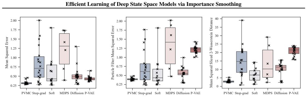
These plots demonstrate that whilst established DSMC methods, Stop-Grad, Soft DPF and MDPS, occasionally converge to a good representation, they suffer from much greater random seed dependence than PVMC. 29 Efficient Learning of Deep State Space Models via Importance Smoothing G.5. Financial time series — generative modelling This final experiment is incl...
work page 2001
-
[20]
layers each with a hidden dimension of 32 (Chen & Li, 2024), with a total of 28,824 learnable parameters. The observation model represents the distribution of log daily returns given the latent state as a mixture of Gaussians. All components of the mixture at all time-steps have the same learned variance, but the weights and locations of each mixture comp...
work page 2024
-
[21]
The DMM similarly represents the proposal by a Gaussian
The total number of learnable parameters of the proposal distribution is 40,408 . The DMM similarly represents the proposal by a Gaussian. Instead of a 1D convolution the DMM parameterises the mean and log covariance by assimilating the results of foward and backwards in time LSTMs (Hochreiter & Schmidhuber, 1997), full details can be found in (Krishnan et al.,
work page 1997
-
[22]
where we artificially suppress the gradient signal due to the prior and dynamic models. For PVMC, DMM, and P-V AE we decrease the suppression from a factor of 0.05 to 1 over the course of training. For Soft DPF it is unclear how one would implement such suppression and it is, to the best of our knowledge, not used in prior work in DPFs. For TCV AE we adop...
work page 2024
discussion (0)
Sign in with ORCID, Apple, or X to comment. Anyone can read and Pith papers without signing in.