REVIEW 5 major objections 8 minor 43 references
Data-Driven Predictive Modeling of Neuronal Dynamics using Long Short-Term Memory
T0 review · 5 major / 8 minor · reviewed 2026-08-14 · deepseek-v4-flash
Pith's one-line read LSTM networks trained for longer prediction horizons forecast neuron spiking more accurately.
desk verdict A competent LSTM surrogate for a CA1 Hodgkin-Huxley model, but the headline horizon trend is confounded by closed-loop iteration count and missing baselines. read the letter →
The pith
A machine-rendered reading of the paper's core claim, the machinery that carries it, and where it could break.
The reading
What carries the argument
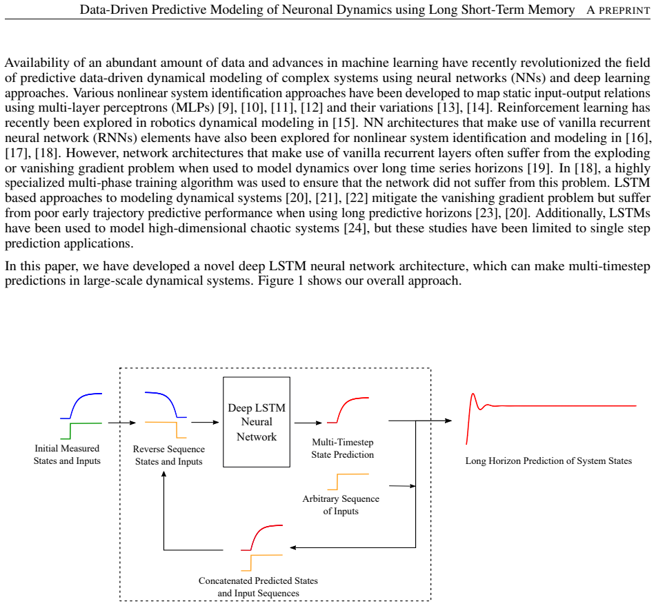
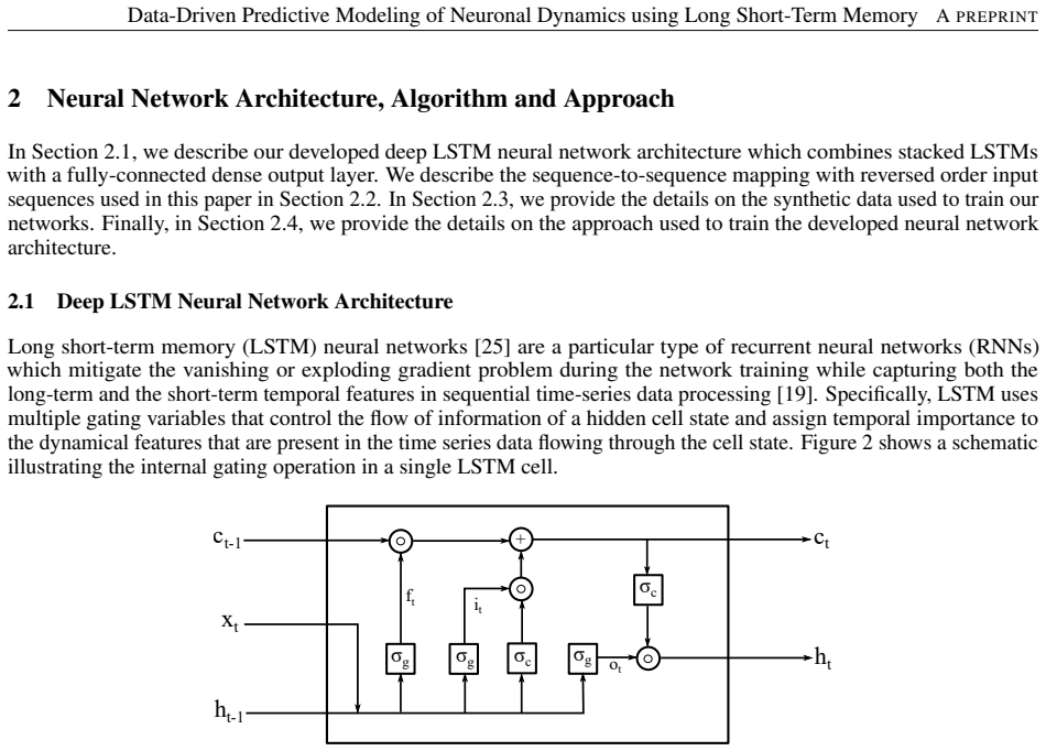
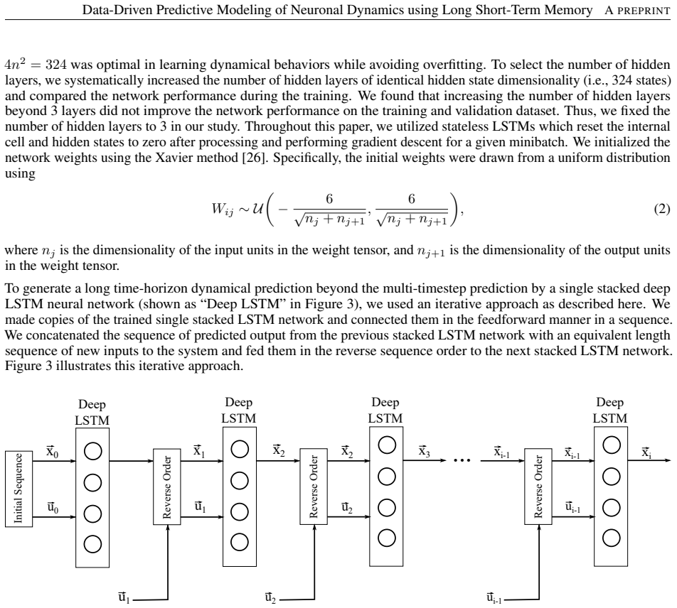
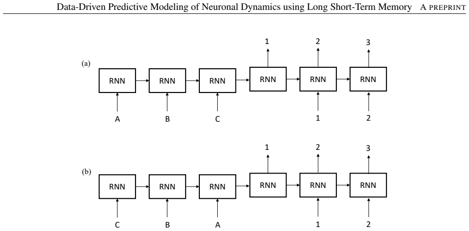
The load-bearing object is a deep LSTM network with three stacked hidden layers of 324 units feeding a single fully connected output layer, trained on simulated traces of the 9-dimensional Hodgkin-Huxley CA1 neuron model. It makes multi-timestep predictions through sequence-to-sequence mapping in which the input sequence is presented in reverse order, so that early inputs correspond to early outputs through short-range dependencies while later inputs map through long-range dependencies; the paper credits this temporal symmetry for improved early-trajectory accuracy. To reach long horizons, copies of the trained network are chained: the predicted output block is concatenated with the next block of inputs and fed, again in reverse order, into the next copy. The iterative chaining plus reversed-order mapping is what carries the claim that a network trained on 20 ms blocks can forecast 500 ms of spiking behavior.
What would settle it
Take a trained $N_p=200$ network and start a 500 ms forecast from a conditioning history that is the true Hodgkin-Huxley trajectory shifted by 1 mV (or corrupted with Gaussian noise of comparable amplitude), then compare RMSE against the clean-history forecast; if the error grows steeply, the reported long-horizon improvement depends on perfectly known initial conditions, and if it does not, the improvement is robust to conditioning error.
Extended reading notes
Core claim
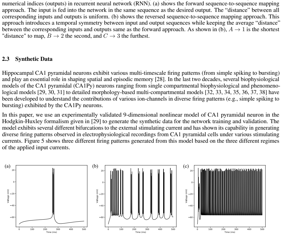
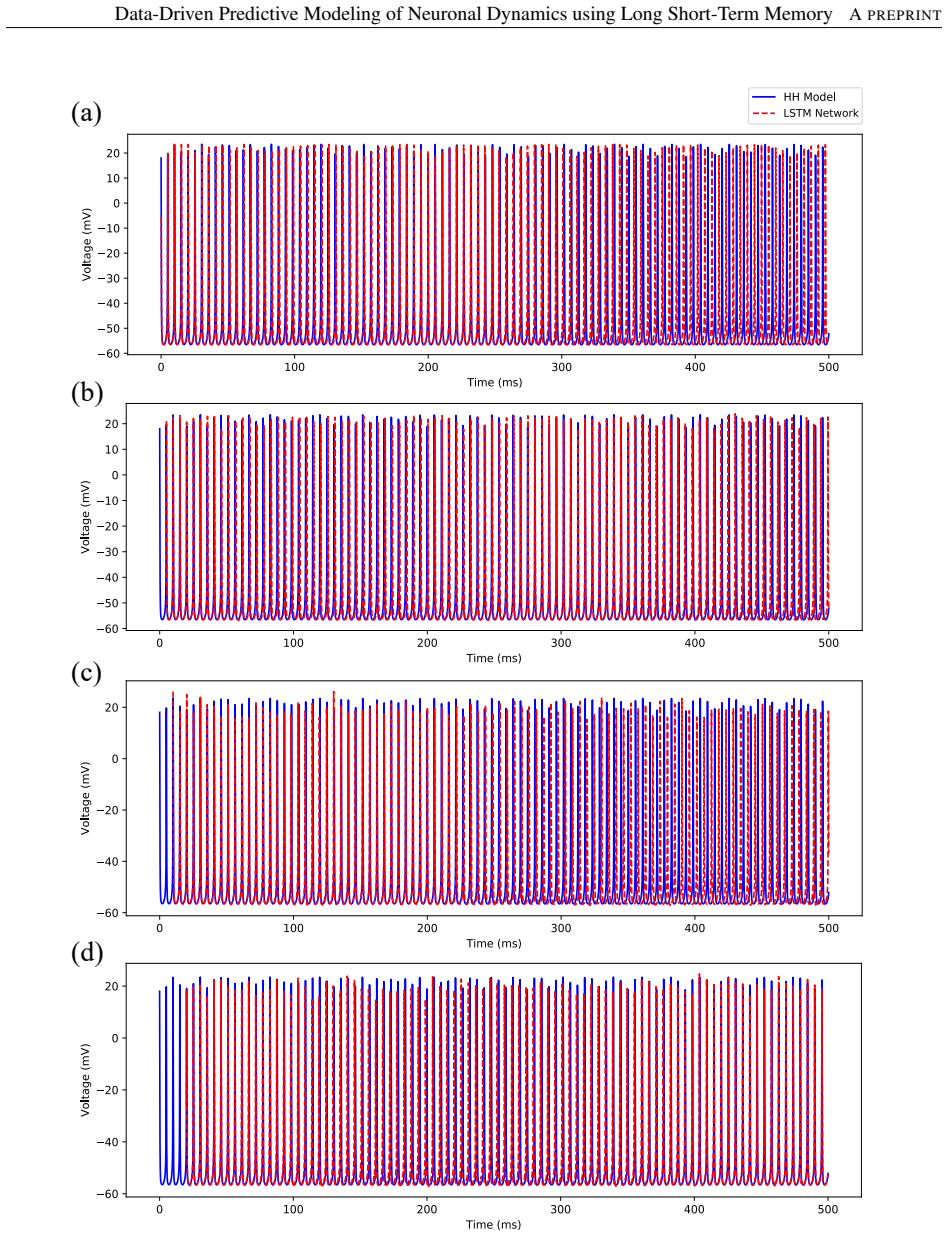
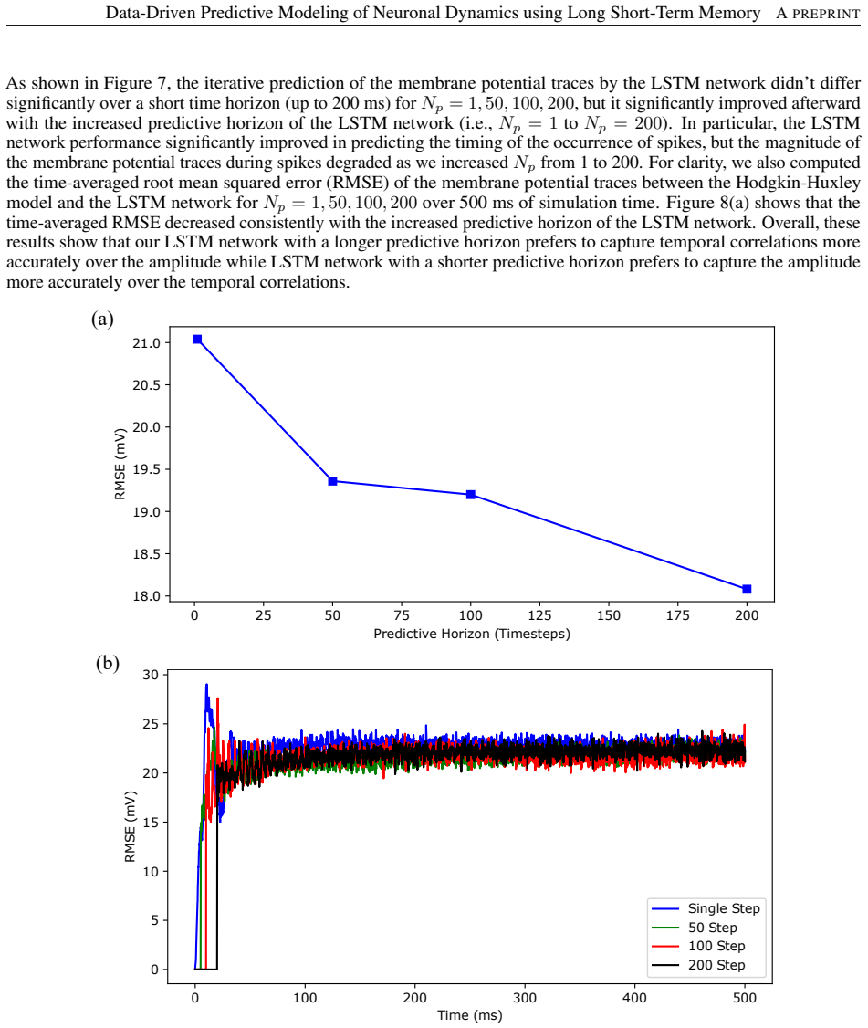
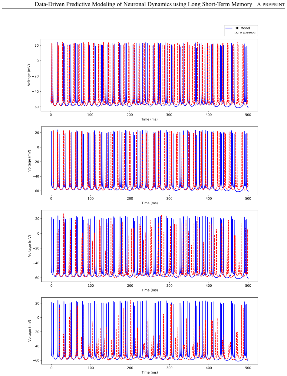
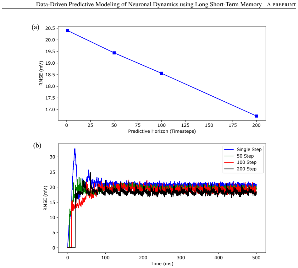
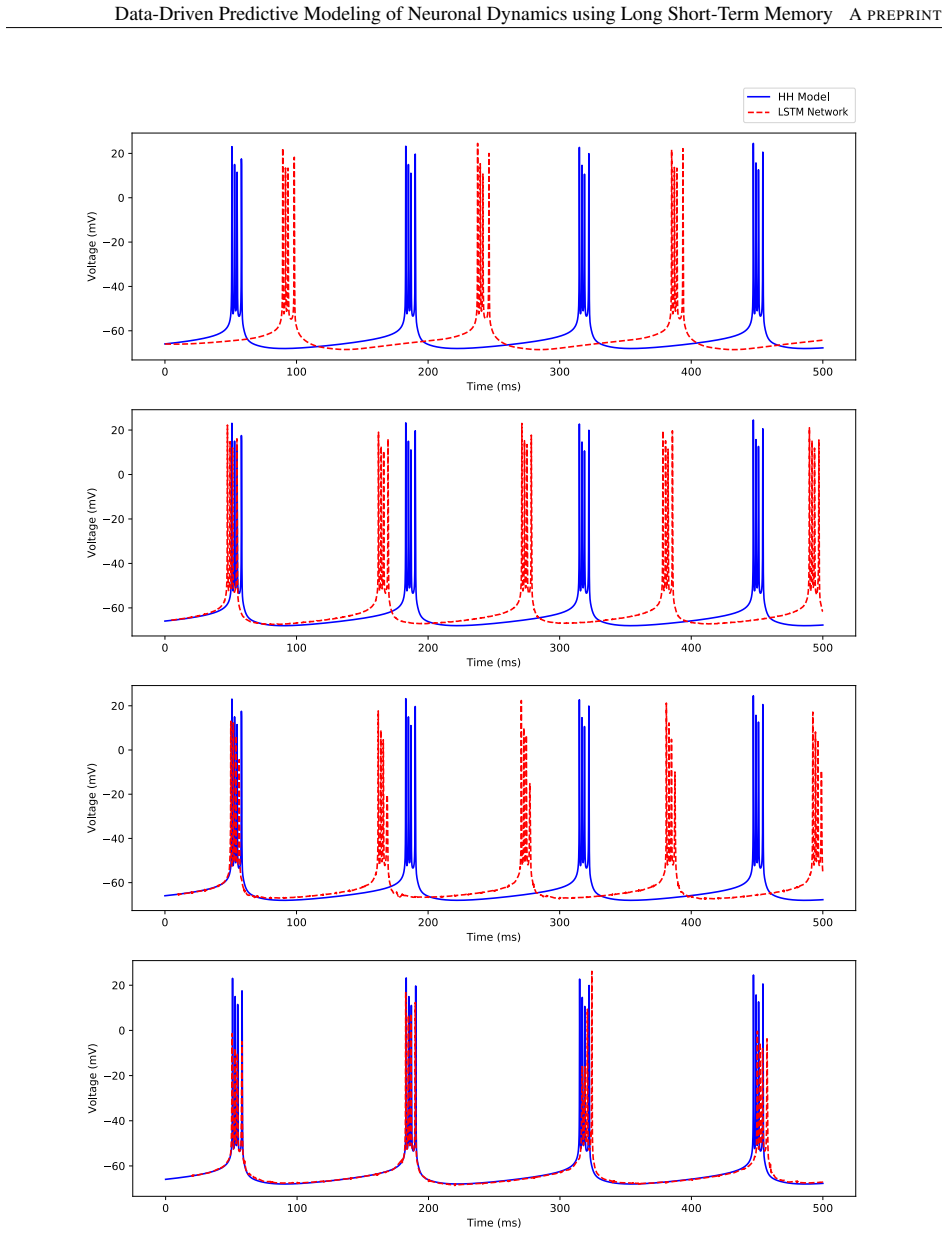
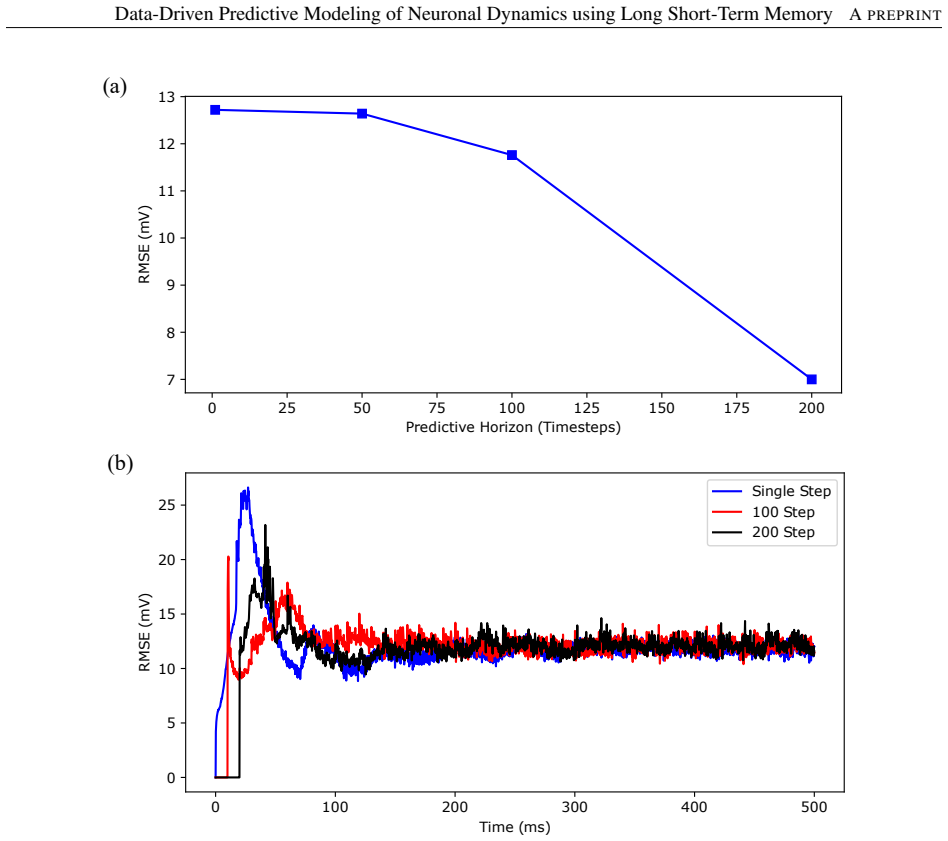
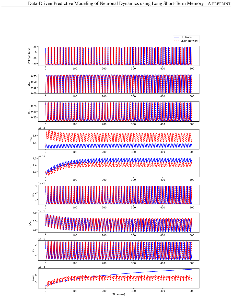
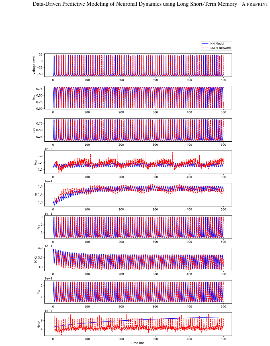
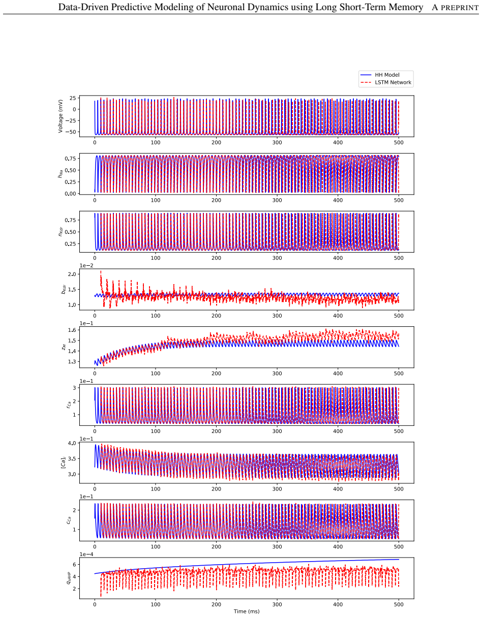
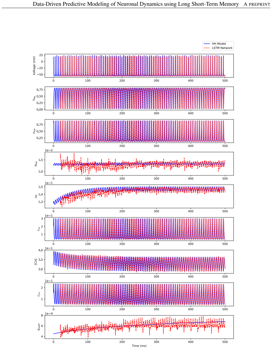
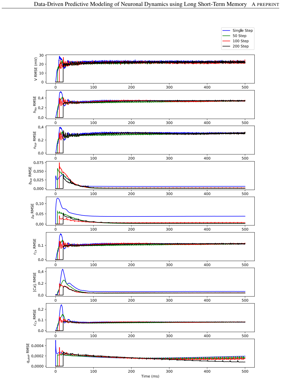
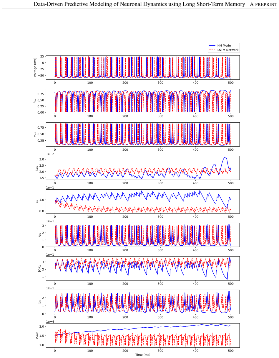
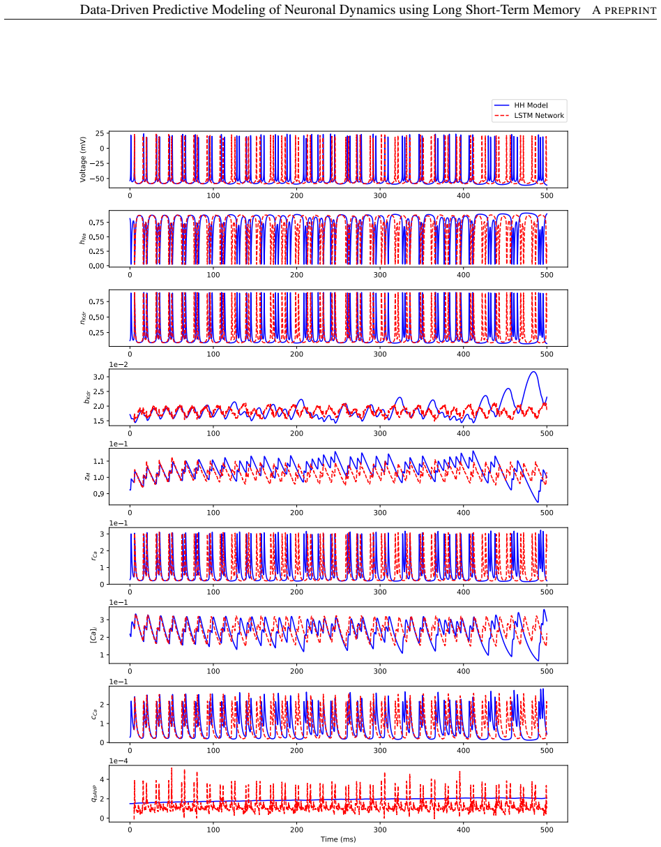
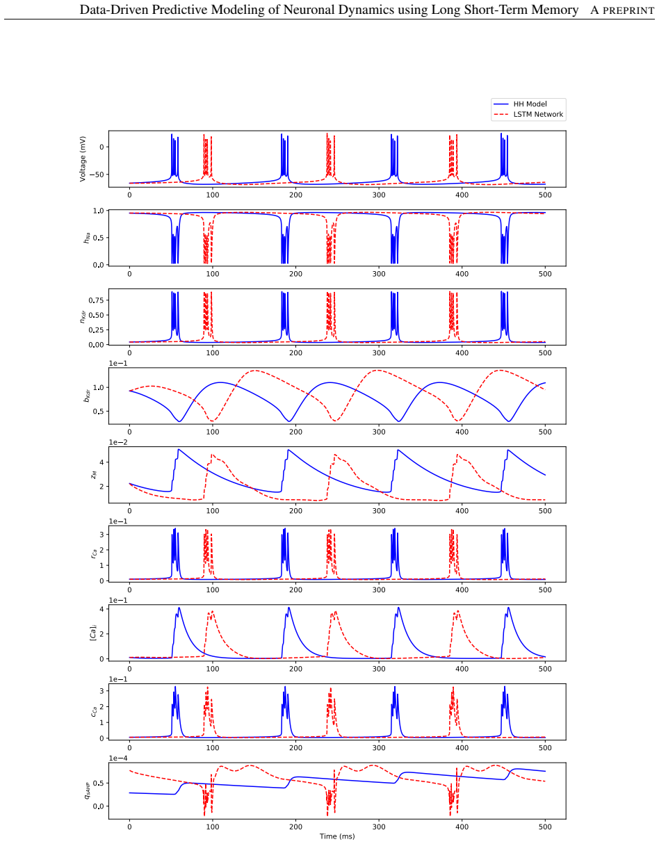
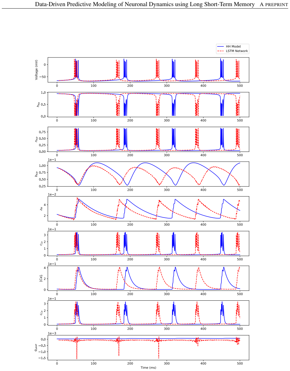
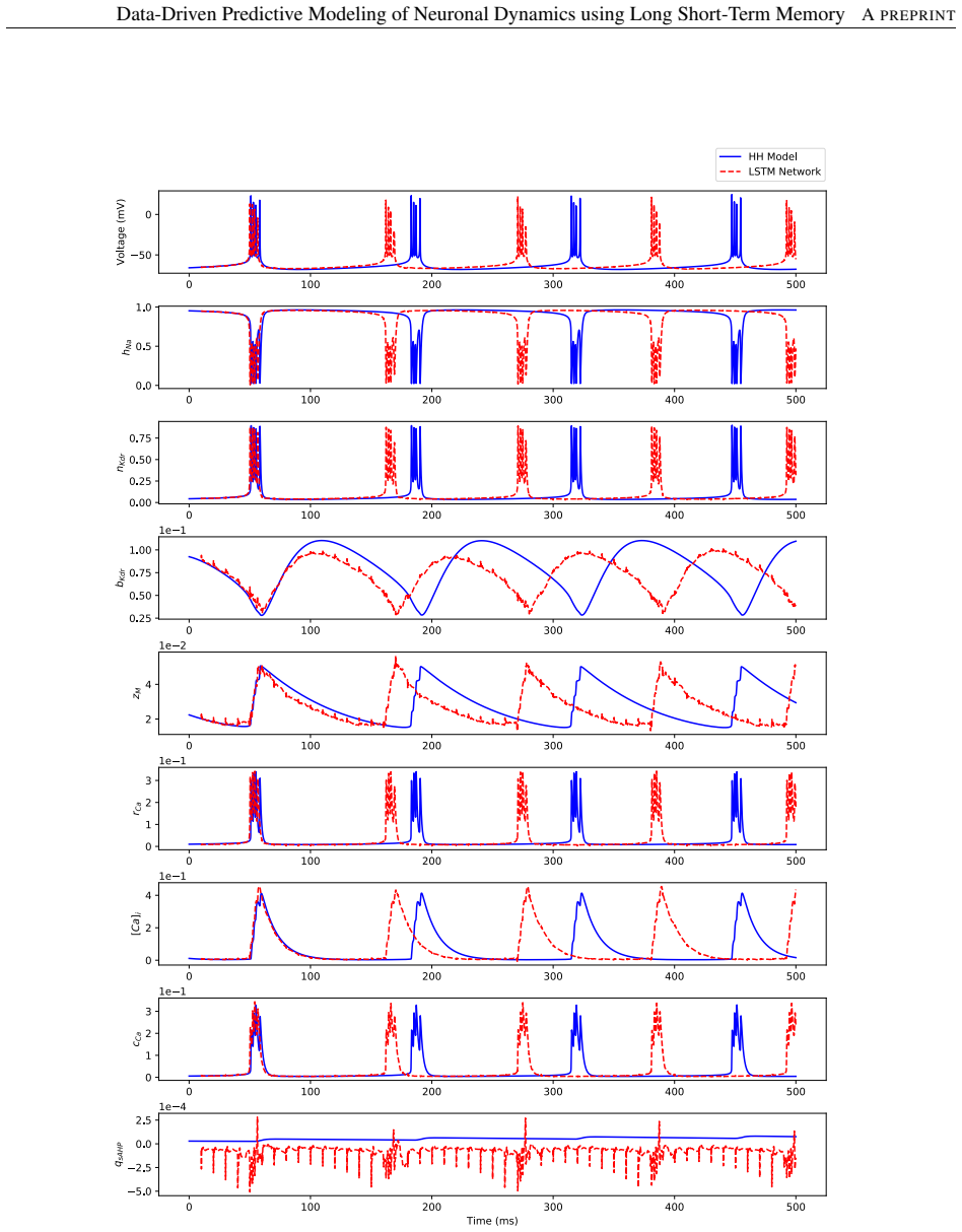
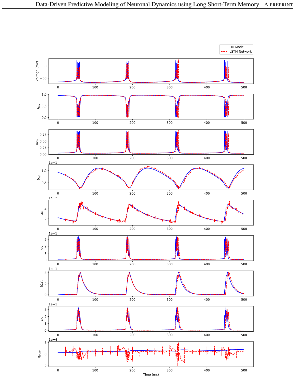
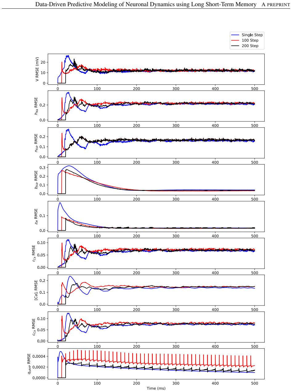
On the paper's own terms, the central discovery is that prediction accuracy improves with the length of the multi-timestep predictive horizon: time-averaged RMSE of the membrane potential decreases consistently as $N_p$ goes from 1 to 50 to 100 to 200 timesteps, in all three dynamical regimes, over 5000 random current-and-initial-condition realizations. Longer-horizon networks track the timing of spikes better, while shorter-horizon networks track spike amplitude better. The regular spiking regime is predicted with high accuracy over the full 500 ms; irregular bursting is captured only over roughly the first 100 ms; regular bursting is captured with reasonable accuracy over about 300 ms for $N_p = 200$. The paper also reports that one gating variable, $q_{sAHP}$, is not reconstructed because its magnitude approaches numerical precision.
Load-bearing premise
The load-bearing premise is that the true Hodgkin-Huxley state trajectory is available as the initial $N_p$-step input sequence for every forecast, so the paper never tests how the network behaves when the conditioning history contains errors or partial observations.
Editorial extensions
If this is right
- In the regular spiking regime, a network trained to predict 20 ms blocks can be iterated over 500 ms with lower RMSE than a network trained for single-step prediction, so longer-horizon training is a viable route to long forecasts.
- Across all three regimes, increasing $N_p$ shifts the error trade-off: spike timing improves while spike amplitude degrades, meaning the loss function directly shapes what the surrogate captures.
- Irregular bursting is not predictable beyond about 100 ms by any of the trained horizons, which sets a concrete limit on neurostimulation control in that regime.
- The slow calcium-activated potassium variable $q_{sAHP}$ is not learned to reasonable accuracy, so the surrogate does not fully reconstruct the 9-dimensional state even when membrane potential traces look right.
- Longer horizons require substantially more offline training cost for the same number of examples, so choosing $N_p$ is a practical trade-off between forecast accuracy and training budget.
Reading between the lines
- Not tested in the paper: corrupting the conditioning sequence with observation noise, then checking whether the $N_p=200$ advantage survives.
- Not tested in the paper: applying the same architecture to a chaotic or aperiodic system, which would show whether the reverse-order benefit generalizes beyond periodic spiking patterns.
- Not tested in the paper: probing horizons beyond $N_p=200$ to see whether the RMSE trend saturates, plateaus, or reverses.
- Not tested in the paper: retraining with norm-1 or weighted norm-2 losses to see if spike amplitude and timing can be recovered together, as the discussion leaves this open.
Signed reviews
Editorial analysis
A structured set of objections, weighed in public.
Referee Report
Summary. The paper proposes a deep LSTM architecture with a single fully connected output layer and reversed-order sequence-to-sequence mapping for multi-step prediction of Hodgkin-Huxley CA1 pyramidal neuron dynamics. The authors train networks with predictive horizons Np = 1, 50, 100, and 200, and evaluate them in closed-loop iterative prediction over 500 ms across three firing regimes: regular spiking, irregular bursting, and regular bursting. The main claim is that time-averaged RMSE decreases as the predictive horizon Np increases. The paper also reports full-state prediction results in Appendix B and discusses limitations in Section 4.
Significance. If the horizon-dependent improvement is genuine and not an artifact of the evaluation protocol, the result would be useful for data-driven surrogate models in control-oriented neurostimulation, because larger multi-step horizons reduce the number of recursive rollouts and may mitigate error accumulation. The paper provides the complete Hodgkin-Huxley model equations in Appendix A and evaluates across three regimes with 5000 realizations, which are strengths. However, the central claim is currently under-supported by the absence of statistical significance tests, baselines, and an ablation separating horizon length from iteration count. The claimed architectural novelty (reverse-order mapping and the single dense output layer) is not directly validated against a forward-order or single-step baseline.
major comments (5)
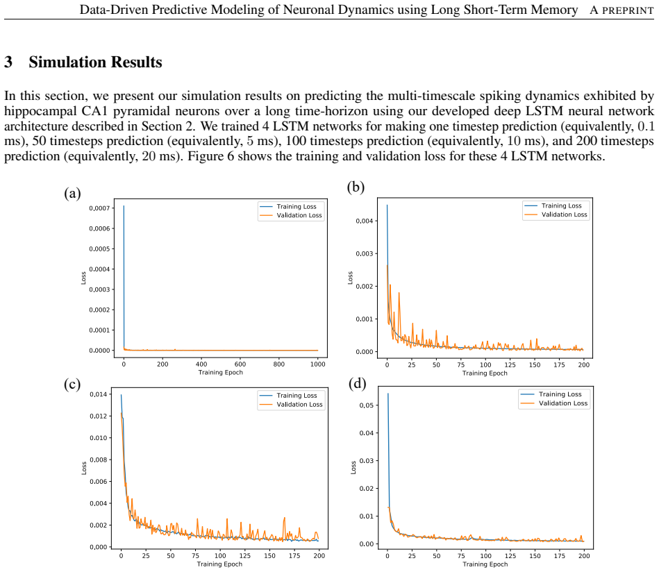
- [Section 2.1, Section 2.4, Figures 7-12] The closed-loop evaluation is confounded with the number of recursive iterations. Section 2.1 states that each Deep LSTM block receives the predicted output sequence from the previous block, while Section 2.4 trains the network by Eq. (4) on true HH state sequences. Over the 500 ms evaluation window, the Np=1 network is rolled out 5000 times, whereas the Np=200 network is rolled out only 25 times. The observed decrease in RMSE with increasing Np may therefore reflect fewer opportunities for feedback-error accumulation rather than better learned dynamics. The manuscript does not report a control that fixes the number of iterations (e.g., re-supplying true states before each block or rolling out the Np=200 network for the same number of steps as Np=1). Without such a control, the abstract's claim that predictions improve with increasing predictive time-horizon is not supported as a property of the learned model.
- [Section 3, Figures 8, 10, 12] The 'decreased consistently' claim is descriptive only. Figures 8(b), 10(b), and 12(b) plot mean RMSE over 5000 realizations without confidence bands, standard deviations, or significance tests, and Figures 8(a), 10(a), and 12(a) compare four horizon values from a single trajectory. No repeated training runs with different seeds are reported, so the reader cannot judge whether the RMSE differences between Np values are larger than training variability. Additionally, no baseline architecture is evaluated: the claimed benefits of the single dense output layer and the reversed-order mapping (Section 2.2) are not tested against a forward-order sequence-to-sequence LSTM or a standard single-step LSTM with feedback. The experimental section therefore does not currently validate either the horizon trend or the architectural novelty.
- [Section 3.3, Figure 12(b)] The regular-bursting RMSE-vs-time panel excludes Np=50, with the text stating that the Np=50 network became unstable for some initial conditions. Since the central claim is that longer horizons uniformly improve accuracy, omitting the Np=50 curve without plotting it or reporting its RMSE prevents the reader from assessing whether the trend is monotone. If Np=50 was unstable, the authors should show the affected trajectories or quantify the failure rate; otherwise the selective exclusion weakens the cross-regime conclusion.
- [Abstract; Sections 3.2, 3.3; Appendix B] The abstract states that the network can predict multi-timescale dynamics 'with reasonable accuracy' and Section 3.1 concludes 'high accuracy over a long-time horizon,' but Sections 3.2 and 3.3 report that in the irregular-bursting regime none of the networks predicted spike timing beyond 100 ms, and in regular bursting the Np=200 network is reasonable only over the first 300 ms. Appendix B also acknowledges that the qsAHP state is not reconstructed. The summary of results should be revised to reflect these stated limitations rather than presenting the regular-spiking result as representative of all regimes.
- [Sections 2.3 and 3] The paper does not state whether the test currents and initial conditions used in Section 3 were excluded from the training set described in Section 2.3. Training currents were sampled uniformly in [0, 3] nA, and test currents are drawn from uniform distributions within subintervals of that range; if there is overlap, the evaluation is not out-of-sample. The authors should specify the splitting procedure and, ideally, ensure that the 50 test currents and the 100 initial conditions per current are disjoint from the training set.
minor comments (8)
- [Abstract] The abstract contains grammatical errors: 'are of interests' should be 'are of interest', and 'from the last several decades' should be 'over the last several decades'.
- [Equation (2)] The Xavier initialization bounds appear to be missing a square root around the denominator; standard Glorot initialization uses ±sqrt(6/(fan_in+fan_out)). Please correct the formula.
- [Equation (4)] The summation index k=0,...,NP and the use of 1/NP suggest the loss averages over NP+1 terms; clarify whether the horizon includes the initial condition or not.
- [Section 2.3] The text says 'we randomly and uniformly drew 50 samples (i.e., 104 data points)'; this arithmetic is unclear, as 50 samples of a 1000-ms trajectory at 0.1 ms would be much larger, and 104 appears to be a typo for 10^4.
- [Appendix A] The state variable z_M is sometimes written as u_KM in the initial conditions list, and the parameter list duplicates θ_c with different values; use consistent notation and check parameter labels.
- [Appendix B.3] The text contains a typo: 'LTSM' should be 'LSTM'.
- [Figures 8(b), 10(b), 12(b)] Consider plotting confidence intervals (e.g., percentiles or standard errors) rather than a single mean curve, since the number of realizations is large enough to make this informative.
- [General] The paper would benefit from a statement on data and code availability; the complete HH model in Appendix A is helpful, but the training and testing pipeline is not documented at the level needed for reproduction.
Circularity Check
No significant circularity: the central horizon-dependence claim is an empirical benchmark of four separately trained networks, not a derivation forced by the training objective or by self-citation.
full rationale
The central claim (Abstract; Section 3.1) that time-averaged RMSE decreases as the predictive-horizon parameter Np increases from 1 to 200 is an empirical comparison of four independently trained LSTM networks, not a quantity derived from the training objective. Equation (4) defines each network's training loss over its own NP, while the reported RMSE in Figures 8, 10, and 12 is evaluated over 500 ms on test currents and initial conditions largely outside the training set; no free parameter is fit to those RMSE curves, and no self-citation is load-bearing. The reverse-order sequence-to-sequence design is credited to an external reference [27]. The evaluation protocol does contain a strong and somewhat ambiguous premise: Section 2.3 assumes the initial output sequence 'is available to the deep LSTM neural network throughout our simulations,' while Figure 3 describes a closed-loop feedforward of predicted outputs. This ambiguity is a validity/robustness concern, not circularity, because even under either reading the decreasing-RMSE trend is not forced by construction. The paper's own Discussion also reports degraded spike-amplitude prediction and poor q_sAHP reconstruction, showing that the results are not definitionally guaranteed.
Assumptions & free parameters
free parameters (5)
- Number of LSTM hidden units per layer =
324 (4n^2 for n=9)
- Number of stacked LSTM layers =
3
- Predictive horizon Np =
1, 50, 100, 200 timesteps
- Adam learning rate =
0.001
- Training epochs =
200 (Np>1), 1000 (Np=1)
assumptions (4)
- domain assumption The Golomb et al. Hodgkin-Huxley model [29] is an experimentally validated ground truth for CA1 pyramidal neuron dynamics
- domain assumption The initial sequence of true states is available to condition every prediction
- domain assumption Constant stimulating currents uniformly sampled in [0,3] nA cover the relevant dynamical regimes
- ad hoc to paper The norm-2 loss equally weighting all 9 states is an appropriate training objective
Cite this review
Pith. "Pith review of Data-Driven Predictive Modeling of Neuronal Dynamics using Long Short-Term Memory." pith.science (2026). https://pith.science/paper/7GRJJYZI
@misc{pith2026190807428,
  author       = {Pith},
  title        = {Pith review of: Data-Driven Predictive Modeling of Neuronal Dynamics using Long Short-Term Memory},
  year         = {2026},
  howpublished = {\url{https://pith.science/paper/7GRJJYZI}},
  note         = {Machine review of arXiv:1908.07428}
}
read the original abstract
Modeling brain dynamics to better understand and control complex behaviors underlying various cognitive brain functions are of interests to engineers, mathematicians, and physicists from the last several decades. With a motivation of developing computationally efficient models of brain dynamics to use in designing control-theoretic neurostimulation strategies, we have developed a novel data-driven approach in a long short-term memory (LSTM) neural network architecture to predict the temporal dynamics of complex systems over an extended long time-horizon in future. In contrast to recent LSTM-based dynamical modeling approaches that make use of multi-layer perceptrons or linear combination layers as output layers, our architecture uses a single fully connected output layer and reversed-order sequence-to-sequence mapping to improve short time-horizon prediction accuracy and to make multi-timestep predictions of dynamical behaviors. We demonstrate the efficacy of our approach in reconstructing the regular spiking to bursting dynamics exhibited by an experimentally-validated 9-dimensional Hodgkin-Huxley model of hippocampal CA1 pyramidal neurons. Through simulations, we show that our LSTM neural network can predict the multi-time scale temporal dynamics underlying various spiking patterns with reasonable accuracy. Moreover, our results show that the predictions improve with increasing predictive time-horizon in the multi-timestep deep LSTM neural network.
Figures
Figures from the paper (24 more)


Reference graph
Works this paper leans on
-
[1]
Dynamics of brain activation during picture naming
R Salmelin, R Hari, OV Lounasmaa, and M Sams. Dynamics of brain activation during picture naming. Nature, 368(6470):463, 1994
work page 1994
-
[2]
The human brain is intrinsically organized into dynamic, anticorrelated functional networks
Michael D Fox, Abraham Z Snyder, Justin L Vincent, Maurizio Corbetta, David C Van Essen, and Marcus E Raichle. The human brain is intrinsically organized into dynamic, anticorrelated functional networks. Proceedings of the National Academy of Sciences, 102(27):9673–9678, 2005
work page 2005
-
[3]
A hierarchy of time-scales and the brain
Stefan J Kiebel, Jean Daunizeau, and Karl J Friston. A hierarchy of time-scales and the brain. PLoS computational biology, 4(11):e1000209, 2008
2008
-
[4]
Cambridge University Press, 2014
Wulfram Gerstner, Werner M Kistler, Richard Naud, and Liam Paninski.Neuronal dynamics: From single neurons to networks and models of cognition. Cambridge University Press, 2014
2014
-
[5]
Multiscale modeling of brain dynamics: from single neurons and networks to mathematical tools
Constantinos Siettos and Jens Starke. Multiscale modeling of brain dynamics: from single neurons and networks to mathematical tools. Wiley Interdisciplinary Reviews: Systems Biology and Medicine, 8(5):438–458, 2016
work page 2016
-
[6]
Dynamic models of large-scale brain activity
Michael Breakspear. Dynamic models of large-scale brain activity. Nature neuroscience, 20(3):340, 2017
work page 2017
-
[7]
Modeling single-neuron dynamics and computations: a balance of detail and abstraction
Andreas VM Herz, Tim Gollisch, Christian K Machens, and Dieter Jaeger. Modeling single-neuron dynamics and computations: a balance of detail and abstraction. science, 314(5796):80–85, 2006
work page 2006
-
[8]
How good are neuron models? Science, 326(5951):379–380, 2009
Wulfram Gerstner and Richard Naud. How good are neuron models? Science, 326(5951):379–380, 2009
work page 2009
Show all 43 references
-
[9]
Neural networks for nonlinear dynamic system modelling and identification
SABS Chen and SA Billings. Neural networks for nonlinear dynamic system modelling and identification. International journal of control, 56(2):319–346, 1992
1992
-
[10]
Nonlinear system identification using neural networks
S Purwar, IN Kar, and AN Jha. Nonlinear system identification using neural networks. IETE journal of research, 53(1):35–42, 2007
2007
-
[11]
Application of feedforward neural networks to dynamical system identification and control
John G Kuschewski, Stefen Hui, and Stanislaw H Zak. Application of feedforward neural networks to dynamical system identification and control. IEEE Transactions on Control Systems Technology, 1(1):37–49, 1993
1993
-
[12]
Long-time predictive modeling of nonlinear dynamical systems using neural networks
Shaowu Pan and Karthik Duraisamy. Long-time predictive modeling of nonlinear dynamical systems using neural networks. Complexity, 2018, 2018
2018
-
[13]
Modeling robot dynamics using dynamic neural networks
Pramod Gupta and Naresh K Sinha. Modeling robot dynamics using dynamic neural networks. IFAC Proceedings Volumes, 30(11):755–759, 1997
1997
-
[14]
Identification of nonlinear dynamic systems using functional link artificial neural networks
Jagdish Chandra Patra, Ranendra N Pal, BN Chatterji, and Ganapati Panda. Identification of nonlinear dynamic systems using functional link artificial neural networks. IEEE transactions on systems, man, and cybernetics, part b (cybernetics), 29(2):254–262, 1999. 15 Data-Driven Pr...
1999
-
[15]
Neural network dynamics for model- based deep reinforcement learning with model-free fine-tuning
Anusha Nagabandi, Gregory Kahn, Ronald S Fearing, and Sergey Levine. Neural network dynamics for model- based deep reinforcement learning with model-free fine-tuning. In 2018 IEEE International Conference on Robotics and Automation (ICRA), pages 7559–7566. IEEE, 2018
2018
-
[16]
Harnessing nonlinearity: Predicting chaotic systems and saving energy in wireless communication
Herbert Jaeger and Harald Haas. Harnessing nonlinearity: Predicting chaotic systems and saving energy in wireless communication. science, 304(5667):78–80, 2004
2004
-
[17]
A recurrent neural network for modelling dynamical systems
Coryn AL Bailer-Jones, David JC MacKay, and Philip J Withers. A recurrent neural network for modelling dynamical systems. network: computation in neural systems, 9(4):531–547, 1998
1998
-
[18]
Deepmpc: Learning deep latent features for model predictive control
Ian Lenz, Ross A Knepper, and Ashutosh Saxena. Deepmpc: Learning deep latent features for model predictive control. In Robotics: Science and Systems. Rome, Italy, 2015
2015
-
[19]
On the difficulty of training recurrent neural networks
Razvan Pascanu, Tomas Mikolov, and Yoshua Bengio. On the difficulty of training recurrent neural networks. In International conference on machine learning, pages 1310–1318, 2013
2013
-
[20]
Multistep prediction of dynamic systems with recurrent neural networks
Nima Mohajerin and Steven L Waslander. Multistep prediction of dynamic systems with recurrent neural networks. IEEE transactions on neural networks and learning systems, 2019
2019
-
[21]
Deep learning-based human-driven vehicle trajectory prediction and its application for platoon control of connected and autonomous vehicles
Lei Lin, Siyuan Gong, Tao Li, and Srinivas Peeta. Deep learning-based human-driven vehicle trajectory prediction and its application for platoon control of connected and autonomous vehicles. In The Autonomous Vehicles Symposium, volume 2018, 2018
2018
-
[22]
Non-linear system modeling using lstm neural networks
Jesús Gonzalez and Wen Yu. Non-linear system modeling using lstm neural networks. IFAC-PapersOnLine, 51(13):485–489, 2018
2018
-
[23]
A new concept using LSTM neural networks for dynamic system identification
Yu Wang. A new concept using LSTM neural networks for dynamic system identification. In 2017 American Control Conference (ACC), pages 5324–5329. IEEE, 2017
2017
-
[24]
Data-driven forecasting of high-dimensional chaotic systems with long short-term memory networks
Pantelis R Vlachas, Wonmin Byeon, Zhong Y Wan, Themistoklis P Sapsis, and Petros Koumoutsakos. Data-driven forecasting of high-dimensional chaotic systems with long short-term memory networks. Proceedings of the Royal Society A: Mathematical, Physical and Engineering Sciences,...
2018
-
[25]
Long short-term memory
Sepp Hochreiter and Jürgen Schmidhuber. Long short-term memory. Neural computation, 9(8):1735–1780, 1997
1997
-
[26]
Understanding the difficulty of training deep feedforward neural networks
Xavier Glorot and Yoshua Bengio. Understanding the difficulty of training deep feedforward neural networks. In Proceedings of the thirteenth international conference on artificial intelligence and statistics, pages 249–256, 2010
2010
-
[27]
Sequence to sequence learning with neural networks
Ilya Sutskever, Oriol Vinyals, and Quoc V Le. Sequence to sequence learning with neural networks. In Advances in neural information processing systems, pages 3104–3112, 2014
2014
-
[28]
CA1 pyramidal cells have diverse biophysical properties, affected by development, experience, and aging
Erin C McKiernan and Diano F Marrone. CA1 pyramidal cells have diverse biophysical properties, affected by development, experience, and aging. PeerJ, 5:e3836, 2017
2017
-
[29]
Contribution of persistent na+ current and m-type k+ current to somatic bursting in ca1 pyramidal cells: combined experimental and modeling study
David Golomb, Cuiyong Yue, and Yoel Yaari. Contribution of persistent na+ current and m-type k+ current to somatic bursting in ca1 pyramidal cells: combined experimental and modeling study. Journal of neurophysiology, 96(4):1912–1926, 2006
1912
-
[30]
A unified model of CA1/3 pyramidal cells: An investigation into excitability
Jakub Nowacki, Hinke M Osinga, Jon T Brown, Andrew D Randall, and Krasimira Tsaneva-Atanasova. A unified model of CA1/3 pyramidal cells: An investigation into excitability. Progress in biophysics and molecular biology, 105(1-2):34–48, 2011
2011
-
[31]
Simple, biologically-constrained CA1 pyramidal cell models using an intact, whole hippocampus context
Katie A Ferguson, Carey YL Huh, Benedicte Amilhon, Sylvain Williams, and Frances K Skinner. Simple, biologically-constrained CA1 pyramidal cell models using an intact, whole hippocampus context. F1000Research, 3, 2014
2014
-
[32]
Arithmetic of subthreshold synaptic summation in a model CA1 pyramidal cell
Panayiota Poirazi, Terrence Brannon, and Bartlett W Mel. Arithmetic of subthreshold synaptic summation in a model CA1 pyramidal cell. Neuron, 37(6):977–987, 2003
2003
-
[33]
Role of ax- onal NaV1
Michel Royeck, Marie-Therese Horstmann, Stefan Remy, Margit Reitze, Yoel Yaari, and Heinz Beck. Role of ax- onal NaV1. 6 sodium channels in action potential initiation of CA1 pyramidal neurons.Journal of neurophysiology, 100(4):2361–2380, 2008
2008
-
[34]
Synapse distribution suggests a two-stage model of dendritic integration in CA1 pyramidal neurons.Neuron, 63(2):171–177, 2009
Yael Katz, Vilas Menon, Daniel A Nicholson, Yuri Geinisman, William L Kath, and Nelson Spruston. Synapse distribution suggests a two-stage model of dendritic integration in CA1 pyramidal neurons.Neuron, 63(2):171–177, 2009
2009
-
[35]
On the mechanisms underlying the depolarization block in the spiking dynamics of CA1 pyramidal neurons
Daniela Bianchi, Addolorata Marasco, Alessandro Limongiello, Cristina Marchetti, Helene Marie, Brunello Tirozzi, and Michele Migliore. On the mechanisms underlying the depolarization block in the spiking dynamics of CA1 pyramidal neurons. Journal of computational neuroscience,...
2012
-
[36]
Fast and accurate low-dimensional reduction of biophysically detailed neuron models
Addolorata Marasco, Alessandro Limongiello, and Michele Migliore. Fast and accurate low-dimensional reduction of biophysically detailed neuron models. Scientific reports, 2(928):1–7, 2012
2012
-
[37]
Dendritic sodium spikes are required for long-term potentiation at distal synapses on hippocampal pyramidal neurons
Yujin Kim, Ching-Lung Hsu, Mark S Cembrowski, Brett D Mensh, and Nelson Spruston. Dendritic sodium spikes are required for long-term potentiation at distal synapses on hippocampal pyramidal neurons. Elife, 4:(e06414) 1–30, 2015
2015
-
[38]
Interneuronal mechanisms of hippocampal theta oscillations in a full-scale model of the rodent CA1 circuit
Marianne J Bezaire, Ivan Raikov, Kelly Burk, Dhrumil Vyas, and Ivan Soltesz. Interneuronal mechanisms of hippocampal theta oscillations in a full-scale model of the rodent CA1 circuit. Elife, 5:(e18566) 1–106, 2016
2016
-
[39]
Generalization of backpropagation with application to a recurrent gas market model
Paul J Werbos. Generalization of backpropagation with application to a recurrent gas market model. Neural networks, 1(4):339–356, 1988
1988
-
[40]
Backpropagation through time: what it does and how to do it
Paul J Werbos et al. Backpropagation through time: what it does and how to do it. Proceedings of the IEEE, 78(10):1550–1560, 1990
1990
-
[41]
A focused backpropagation algorithm for temporal
Michael C Mozer. A focused backpropagation algorithm for temporal. Backpropagation: Theory, architectures, and applications, 137, 1995
1995
-
[42]
Adam: A method for stochastic optimization
Diederik P Kingma and Jimmy Ba. Adam: A method for stochastic optimization. arXiv preprint arXiv:1412.6980, 2014. A Hodgkin-Huxley Model of CA1 Pyramidal Neuron Dynamics We used the following Hodgkin-Huxley model of CA1 pyramidal neuron from [29] to demonstrate the efficacy of ...
2014 arXiv
-
[43]
HH Model
across all the states exceptqsAHP for the similar reason we provided for the regular spiking and irregular bursting regimes. More importantly, the LTSM network predicted the temporal correlations with high accuracy over the time- 19 Data-Driven Predictive Modeling of Neuronal ...
Reviewed August 14, 2026 · model on record in the stance chip above.
Discussion (0). Continue with ORCID to comment.