REVIEW 3 major objections 6 minor 52 references
Visual Graph Arena: Evaluating Visual Conceptualization of Vision and Multimodal Large Language Models
T0 review · 3 major / 6 minor · reviewed 2026-08-07 · deepseek-v4-flash
Pith's one-line read On Visual Graph Arena, humans score 88–100 percent while vision and multimodal LLMs fail at graph isomorphism and most other tasks.
desk verdict A useful new benchmark for layout-shift visual graph reasoning, but the headline claim about missing conceptualization is not established because the design never rules out vision-encoder parsing failure. read the letter →
The pith
A machine-rendered reading of the paper's core claim, the machinery that carries it, and where it could break.
The reading
What carries the argument
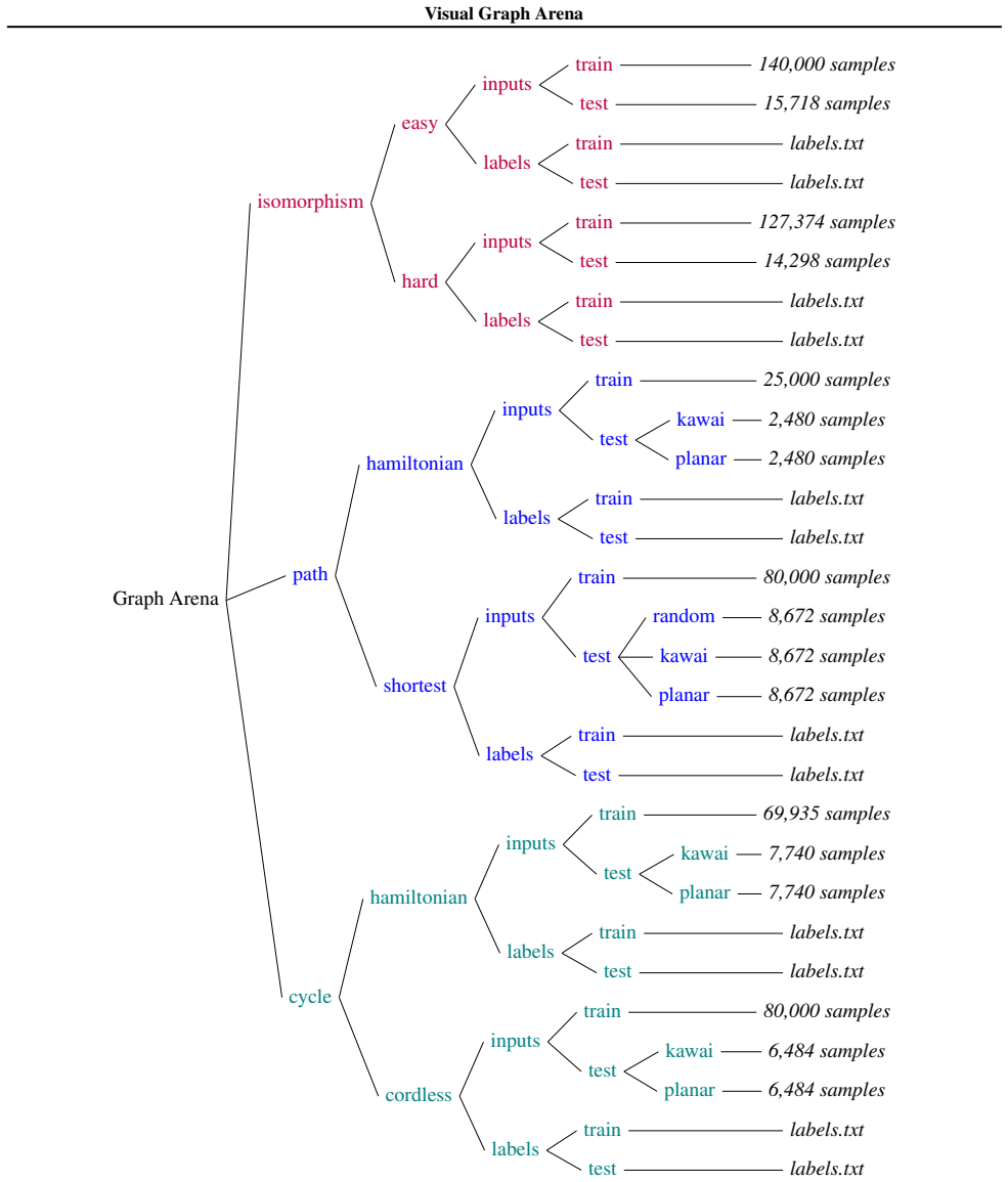
The load-bearing mechanism is the training/test layout split: graphs are rendered in one layout (Kamada-Kawai or random) for training and in a different layout (planar, Kamada-Kawai, or random) for testing, so any above-chance performance requires recognizing the concept rather than memorizing pixel patterns. The six tasks operationalize conceptualization as classification problems: yes/no isomorphism with an easy random-foil and hard degree-equivalent-foil version, yes/no Hamiltonian path and Hamiltonian cycle presence, and four-choice shortest-path and biggest-chordless-cycle lengths. Human performance on the same images supplies the reference level that defines what conceptualization should look like.
What would settle it
Train the same vision encoders on VGA for substantially more than 10 epochs, or provide them with explicit node and edge coordinate supervision, and test on the planar-layout splits. If accuracy on isomorphism jumps to near-human levels, the reported failure is a layout-parsing or training-budget problem rather than a missing conceptual invariant.
Extended reading notes
Core claim
On the paper's own terms, the discovery is that visual conceptualization—recognizing a graph property regardless of how the graph is drawn—is present in human subjects and largely absent from current AI systems. Across the six VGA tasks, vision models fine-tuned for ten epochs performed at chance on easy and hard isomorphism, and only modestly above chance on Hamiltonian path, shortest path, Hamiltonian cycle, and chordless cycle tasks. Multimodal LLMs, including GPT-o1, GPT-4o, and Claude 3.5 Sonnet, mostly performed at or near random, with GPT-o1's partial success on Hamiltonian cycles traceable to leaf-node detection rather than graph reasoning. The paper frames these results as showing that models display pseudo-intelligent pattern matching rather than genuine understanding.
Load-bearing premise
The load-bearing premise is that near-random accuracy on test graphs drawn in a new layout reflects a lack of conceptual understanding, rather than an inability to parse that unfamiliar drawing style.
Editorial extensions
If this is right
- Any model trained on VGA's training splits can be scored for layout transfer by comparing its accuracy on the different-layout test splits, giving a direct measure of representation-invariant visual reasoning.
- Because humans reach 88–100 percent accuracy, the benchmark supplies a concrete performance target that current models do not meet.
- GPT-o1's Hamiltonian-cycle accuracy being tied to leaf-node detection means above-chance scores on graph tasks should not be taken as genuine understanding without checking for shortcut cues.
- Datasets and training schemes aimed at human-like visual understanding can use VGA's layout split as a curriculum signal, since the bottleneck appears to be transfer across visual form rather than graph-problem difficulty.
Reading between the lines
- A natural next experiment would apply the same layout-split protocol to molecular drawings and circuit diagrams; the paper's own framing suggests the failure pattern should recur wherever the same structure can be drawn in many ways.
- The two anomalies (middle scores and easier-worse) can be used as a general diagnostic: any atomic perceptual task where a model scores in the middle and does worse on easy items is likely being solved via shortcut features rather than concept knowledge.
- The 10-epoch fine-tuning budget leaves open that stronger encoders, higher-resolution input, or explicit layout augmentation might narrow or close the gap, which would shift the explanation from missing conceptualization to insufficient invariance training.
Editorial analysis
A structured set of objections, weighed in public.
Referee Report
Summary. The paper introduces the Visual Graph Arena (VGA), a benchmark of six graph tasks (easy and hard isomorphism, Hamiltonian path, shortest path, Hamiltonian cycle, biggest chordless cycle) in which the training and test images use different graph layouts (e.g., Kamada-Kawai vs. planar) to test whether models recognize the same graph concept across visual form. The authors fine-tune several vision models (ViT, Swin, ConvNeXt, SigLIP, DINOv2) on the tasks and evaluate MLLMs (GPT-4o, GPT-o1, Claude 3.5 Sonnet, etc.) in zero-shot settings. The reported results show that humans achieve 88–100% accuracy, while vision models fail or perform modestly on cross-layout tests, and most MLLMs perform near chance. The paper interprets these failures as evidence of a lack of 'conceptualization' and of 'pseudo-intelligent pattern matching' rather than genuine understanding.
Significance. If the benchmark is a valid operationalization of visual conceptualization, the results are striking and would constitute a useful diagnostic dataset for layout-invariant visual reasoning. The dataset is large (27k–150k training samples per task) and the layout-shift protocol is a reasonable way to test representation-invariant reasoning. The inclusion of a human baseline is a strength, as is the attempt to isolate path, cycle, and isomorphism concepts. The central negative findings—near-chance performance on cross-layout isomorphism and limited success on other tasks—are broadly consistent across architectures and are likely to be of interest to the vision and multimodal LLM communities. However, the paper's stronger interpretive claims (absence of conceptualization, pseudo-intelligence) rest on assumptions that are not explicitly validated by the experiments as reported.
major comments (3)
- [§3.2, §4.1, Appendix C] The central inference—that near-chance cross-layout accuracy demonstrates a lack of representation-invariant conceptualization—requires that the vision models can actually parse the test-layout graphs into nodes and edges. The paper never reports a same-layout control: no model is trained on planar-rendered graphs and tested on planar-rendered graphs, or trained on Kamada-Kawai and tested on Kamada-Kawai. Without such a control, the failure could be attributed to the vision encoder's inability to extract nodes and edges from planar drawings (different edge lengths, crossing patterns, and white-space statistics) rather than to an absence of abstract graph reasoning. Please add the missing control experiments or explicitly weaken the conceptualization claim to a claim about layout-transfer robustness.
- [§4.1 and Appendix C] The evaluation protocol violates test-set independence: the paper states that 'we report the best validation accuracy achieved during the training epochs' and that 'the best-performing model on the test set was selected for each task and architecture combination.' Tuning model selection on the test set inflates the reported numbers and makes the benchmark results not reproducible as unbiased estimates. The authors should either use a held-out validation set for early stopping and model selection, or report the last-epoch model's test accuracy, and then report a single, unselected test evaluation.
- [§5.1 and §5.3, Table 3] The interpretation of the confusion pattern in Table 3 as evidence of 'pseudo-intelligent pattern matching' is not supported by the data. The 'atomic-task' framing in §5.1 is not justified: shortest-path length is not an atomic skill that an agent either knows completely or not at all, so intermediate accuracy is not anomalous. Moreover, the confusion between lengths 1 and 2 could plausibly arise from a partial ability to count edges or from perceptual errors in the provided graph drawings. The paper should either provide additional control experiments (e.g., testing GPT-o1 on the same planar graph without the node-marking task) or temper the pseudo-intelligence claim to a more descriptive statement about the observed failure modes.
minor comments (6)
- [§4, 'Humans'] The human baseline uses only 15 subjects and 24 questions total (four per task). Please report the standard errors or confidence intervals and clarify whether each subject answered all 24 questions; the current sentence is ambiguous.
- [Table 2] The 'FAIL' entries are said to indicate near-random performance, but exact numbers are not reported. Please replace the label with the actual accuracy (or a range) so readers can verify that the performance is at chance.
- [§5.1] The examples used to motivate the 'Middle-Score Anomaly' (e.g., recognizing numbers ending in zero) are not analogous to the graph tasks, since the graph tasks admit degrees of partial knowledge. Clarify the scope of the anomaly definition.
- [§3.2, §4.1, Figure 8, Conclusions] Several typos appear: 'Haminltonian' in §3.2, 'Visaul' in §4.1, 'cordless' in Figure 8, and 'designed designed' in the Conclusions. Please correct these.
- [Figure 10 caption] The caption of Figure 10 says 'examples of the easy isomorphism task' but the figure is in the Hard Isomorphism subsection and likely shows hard examples. Please correct the caption.
- [Appendix A and Abstract] The dataset URL is given as vga.csail.mit.edu in the abstract but visualgrapharena.com in Appendix A. Please unify the URL and verify that both lead to the same resource.
Circularity Check
No significant circularity: the paper reports measured benchmark performance rather than deriving predictions from fitted inputs.
full rationale
This paper is an empirical benchmark paper, not a derivation. Its central claims are statements about measured model performance on a newly constructed dataset, and no predicted quantity is produced by fitting a parameter and then renaming that fit as a prediction. The vision models are fine-tuned on rendered graphs in one layout and tested on held-out graphs in another layout; the reported accuracies are test-set measurements, not quantities forced by construction. The 'conceptualization' construct is explicitly defined as the ability to recognize and reason about the same concept across representational variations, so using layout variation as the test condition is an operationalization of that definition rather than a circular reduction. There are no load-bearing self-citations: references to Kamada-Kawai and Tay et al. are used only for graph-drawing layouts and for the term 'FAIL', respectively. The later 'pseudo-intelligent pattern matching' interpretation is an abductive reading of the observed confusion-matrix anomalies, not a step that reduces to the paper's own inputs. Even if the operationalization is debatable, no equation or fitted parameter makes the conclusion equivalent to the input by construction. The benchmark is also self-contained against external human baselines, which provide independent empirical content. I therefore find no specific circular step that can be quoted and exhibited as a reduction.
Assumptions & free parameters
free parameters (6)
- Number of nodes per graph =
8-9
- Shortest path answer classes =
1, 2, 3, 4
- Chordless cycle answer classes =
3, 4, 5, 6
- Train/test layout pairing =
Kamada-Kawai (train) vs planar (test) for path and cycle tasks; random (train) vs random/KK/planar (test) for shortest…
- Degree-equivalent false pairs in hard isomorphism =
degree-equivalent
- Training set size per task =
25,000 to 140,000
assumptions (5)
- domain assumption Graph isomorphism, Hamiltonian path/cycle, and chordless-cycle concepts are visually recognizable in 8-9 node drawings at levels humans can solve.
- domain assumption A vision model that understands a concept should transfer across layouts when fine-tuned on one layout.
- domain assumption The train/test splits prevent graph overlap (no graph appears in both splits).
- domain assumption The MLLM evaluation with 100 samples per task is sufficient to detect conceptual ability.
- domain assumption Pre-trained vision backbones can learn graph visual reasoning from 10 epochs of fine-tuning on up to 140,000 images.
invented entities (1)
-
pseudo-intelligence
Cite this review
Pith. "Pith review of Visual Graph Arena: Evaluating Visual Conceptualization of Vision and Multimodal Large Language Models." pith.science (2026). https://pith.science/paper/7UULODPI
@misc{pith2026250606242,
  author       = {Pith},
  title        = {Pith review of: Visual Graph Arena: Evaluating Visual Conceptualization of Vision and Multimodal Large Language Models},
  year         = {2026},
  howpublished = {\url{https://pith.science/paper/7UULODPI}},
  note         = {Machine review of arXiv:2506.06242}
}
read the original abstract
Recent advancements in multimodal large language models have driven breakthroughs in visual question answering. Yet, a critical gap persists, `conceptualization'-the ability to recognize and reason about the same concept despite variations in visual form, a basic ability of human reasoning. To address this challenge, we introduce the Visual Graph Arena (VGA), a dataset featuring six graph-based tasks designed to evaluate and improve AI systems' capacity for visual abstraction. VGA uses diverse graph layouts (e.g., Kamada-Kawai vs. planar) to test reasoning independent of visual form. Experiments with state-of-the-art vision models and multimodal LLMs reveal a striking divide: humans achieved near-perfect accuracy across tasks, while models totally failed on isomorphism detection and showed limited success in path/cycle tasks. We further identify behavioral anomalies suggesting pseudo-intelligent pattern matching rather than genuine understanding. These findings underscore fundamental limitations in current AI models for visual understanding. By isolating the challenge of representation-invariant reasoning, the VGA provides a framework to drive progress toward human-like conceptualization in AI visual models. The Visual Graph Arena is available at: \href{https://vga.csail.mit.edu/}{vga.csail.mit.edu}
Figures


Figures from the paper (22 more)




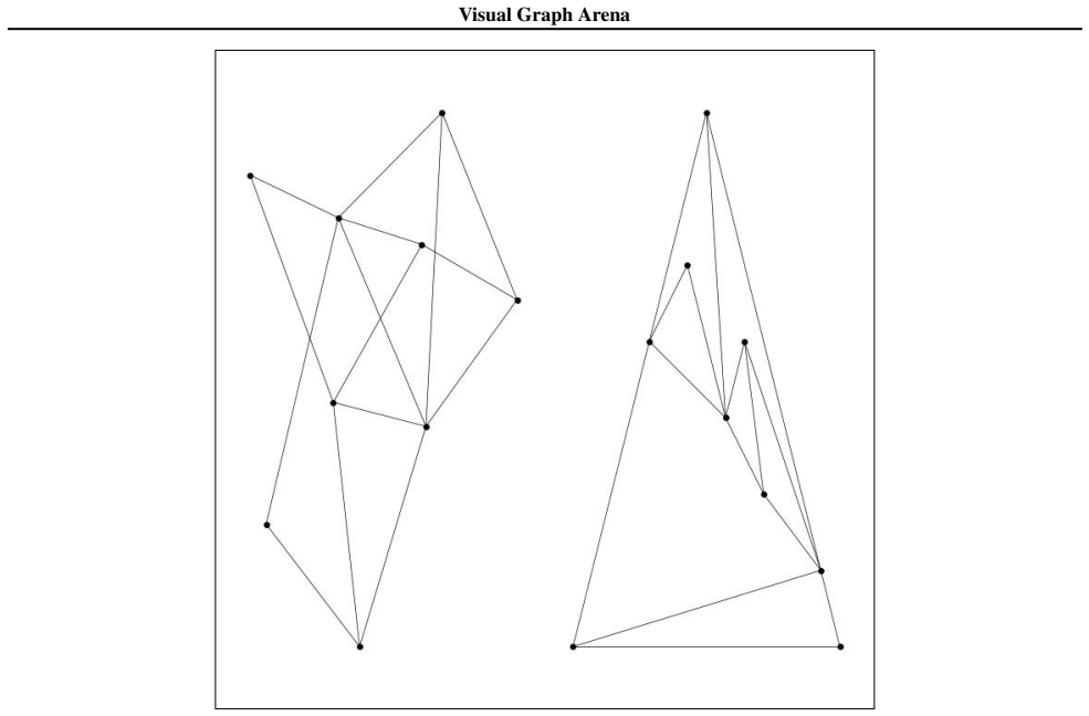


Reference graph
Works this paper leans on
-
[1]
Number of vertices: Both graphs have the same number of vertices
-
[2]
Goyal, Y ., Khot, T., Summers-Stay, D., Batra, D., and Parikh, D
URL https://openreview.net/forum? id=LdRZ9SFBku. Goyal, Y ., Khot, T., Summers-Stay, D., Batra, D., and Parikh, D. Making the v in vqa matter: Elevating the role of image understanding in visual question answer- ing. In Proceedings of the IEEE conference on computer vision and pattern recognition, pp. 6904–6913, 2017. Guetta, N. B., Slobodkin, A., Maimon,...
work page 2017
-
[3]
URL https://openreview.net/forum? id=hwbRjslR5N. Gupta, T. and Kembhavi, A. Visual programming: Compo- sitional visual reasoning without training. In Proceedings of the IEEE/CVF Conference on Computer Vision and Pattern Recognition, pp. 14953–14962, 2023. Han, C., Mao, J., Gan, C., Tenenbaum, J., and Wu, J. Vi- sual concept-metaconcept learning. Advances ...
arXiv 2023
-
[4]
URL https://openreview.net/forum? id=loJM1acwzf. Morris, C., Kriege, N. M., Bause, F., Kersting, K., Mutzel, P., and Neumann, M. Tudataset: A collection of bench- mark datasets for learning with graphs. arXiv preprint arXiv:2007.08663, 2020. Murphy, R., Srinivasan, B., Rao, V ., and Ribeiro, B. Re- lational pooling for graph representations. In Interna- t...
arXiv 2007
-
[5]
Go down to the bottom point of the rightmost triangle
-
[6]
Move up to the right point of that triangle
-
[7]
Number of edges: Both graphs also have the same number of edges
-
[8]
Vertex degrees: The degrees of corresponding vertices (number of edges connected to each vertex) should be the same. However, upon visual inspection, the structure of the graphs seems to differ significantly. The graph on the right has a more symmetrical structure, while the graph on the left appears more irregular. Specifically, the arrangement of connec...
Show all 52 references
-
[9]
The left graph is more densely interconnected, with multiple triangles and a more compact shape
-
[10]
The right graph has a more stretched out, less symmetrical structure
-
[11]
The degree distribution (number of edges connected to each vertex) seems different between the two graphs
-
[12]
These structural differences suggest that there is no one-to-one mapping that could transform one graph into the other while preserving all connections
The left graph appears to have more cycles than the right graph. These structural differences suggest that there is no one-to-one mapping that could transform one graph into the other while preserving all connections. Given these observations, my conclusion is that these graph...
-
[13]
The same number of vertices
-
[14]
The same number of edges
-
[15]
Equivalent connectivity between corresponding pairs of vertices Comparing the two given graphs:
-
[16]
So this condition is satisfied
Number of vertices: Both graphs appear to have 6 vertices each. So this condition is satisfied
-
[17]
Edge count matches
Number of edges: I count 9 edges in the graph on the left, and 9 edges in the graph on the right as well. Edge count matches
-
[18]
We’d need to find a one-to-one mapping between the vertices of the two graphs, such that the edge connections are preserved
Vertex connectivity: This is trickier to verify visually. We’d need to find a one-to-one mapping between the vertices of the two graphs, such that the edge connections are preserved. One potential mapping: Left graph vertex (from top) 1 → 1, 2 → 2, 3 → 6, 4 → 5, 5 → 4, 6 → 3 o...
-
[19]
Visit all 9 vertices
-
[20]
Use only existing edges
-
[21]
Return to the starting point
-
[22]
• The graph is not fully connected - it has a “pinched” middle section
Visit each vertex only once (except the start/end) Looking at the graph structure: • There are several vertices with only two connections, which limits path options. • The graph is not fully connected - it has a “pinched” middle section. • There’s no obvious circular path that...
-
[23]
The graph has 6 vertices
-
[24]
Each vertex has a degree (number of edges connected to it) of at least 2
-
[25]
induced cycle,
It appears that we can trace a path that visits each vertex exactly once and returns to the starting point. One possible Hamiltonian cycle in this graph could be: Start at any vertex, move to an adjacent vertex, then continue moving to unvisited adjacent vertices until all ver...
-
[26]
Identify all cycles: We need to identify all the possible cycles in the graph
-
[27]
Determine if they are chordless: For each cycle, check if there are any extra edges (chords) connecting non-consecutive vertices in the cycle. Observation from the Image: Looking at the graph, a few potential cycles stand out: • Cycle 1: Going through five points that seem to ...
-
[28]
The cycle involving the five vertices appears to be the largest cycle
-
[29]
Conclusion: The biggest chordless cycle in this graph consists of 5 vertices
There are no additional edges (chords) connecting non-consecutive vertices in this cycle, making it a chordless cycle. Conclusion: The biggest chordless cycle in this graph consists of 5 vertices. Thus, the final answer is 5 . Claude 3.5 Sonnet Output: To find the biggest chor...
-
[30]
First, I’ll identify all cycles in the graph
-
[31]
Then, I’ll check each cycle to see if it has any chords (edges connecting non-adjacent vertices within the cycle)
-
[32]
induced”) cycle is to look around the “outer rim
Among the chordless cycles, I’ll determine the largest one. After analyzing the graph: • There are several triangles (3-cycles), but these are too small to be the answer. • I can see a few 4-cycles, but upon closer inspection, they all have chords. • The largest cycle I can fi...
-
[33]
I identified the vertices and observed the connections between them
-
[34]
Given the structure of the graph, it appears that there is no such path that visits every vertex exactly once without retracing any edge or missing any vertex
I checked if there’s a path that visits every vertex exactly once. Given the structure of the graph, it appears that there is no such path that visits every vertex exactly once without retracing any edge or missing any vertex. Final answer: No 30 Visual Graph Arena Claude 3.5 ...
-
[35]
Begin at the leftmost point
-
[36]
Move right to the next point
-
[37]
Go up to the top of the leftmost triangle
-
[38]
Move right to the center point of the graph
-
[41]
Go to the top point of the rightmost triangle
-
[42]
Therefore, the graph does have a Hamiltonian path
End at the uppermost point of the graph This path visits all 8 vertices exactly once, without repeating any vertex. Therefore, the graph does have a Hamiltonian path. Yes Claude 3 Opus Output: To determine whether the given graph has a Hamiltonian path, I’ll analyze its struct...
-
[43]
Start from the square node on the left side of the graph
-
[44]
There is a direct connection to the node above it
-
[45]
Therefore, the shortest path consists of two edges
From this node, there is a connection to the square node on the right side. Therefore, the shortest path consists of two edges. The final answer is 2 . 32 Visual Graph Arena Claude 3.5 Sonnet Output: To find the shortest path between the two square nodes in this graph, I’ll co...
-
[46]
A direct path that goes through the center node of the graph
-
[47]
The direct path through the center is clearly shorter
A path that follows the outer edges of the graph. The direct path through the center is clearly shorter. It requires traversing only 2 edges:
-
[48]
From the first square node to the center node
-
[49]
Therefore, the shortest path between the two square nodes in this graph is 2
From the center node to the second square node The path along the outer edges would require traversing at least 3 edges. Therefore, the shortest path between the two square nodes in this graph is 2 . Claude 3 Opus Output: The image shows a graph with 6 nodes, where 2 nodes are...
-
[50]
Starting from the top square node, there are two possible paths: down-left or down-right
-
[51]
Following the down-left path: Square → Circle → Square This path has a length of 2 edges
-
[52]
Therefore, the shortest path between the two square nodes goes through the down-left path, with a length of 2 edges
Following the down-right path: Square → Circle → Circle → Circle → Square This path has a length of 4 edges. Therefore, the shortest path between the two square nodes goes through the down-left path, with a length of 2 edges. The shortest path between the two square nodes is 2...
-
[2021]
The image presented contains a graph. Please transcribe this graph’s adjacency matrix
URL https://openreview.net/forum? id=qVyeW-grC2k. Wang, K., Pan, J., Shi, W., Lu, Z., Ren, H., Zhou, A., Zhan, M., and Li, H. Measuring multimodal mathematical reasoning with MATH-vision dataset. In The Thirty-eight Conference on Neural Information Processing Systems Datasets ...
2024 arXiv
-
[2024]
Dosovitskiy, A., Beyer, L., Kolesnikov, A., Weissenborn, D., Zhai, X., Unterthiner, T., Dehghani, M., Minderer, M., Heigold, G., Gelly, S., Uszkoreit, J., and Houlsby, N
URL https://openreview.net/forum? id=YMAU2kJgzY. Dosovitskiy, A., Beyer, L., Kolesnikov, A., Weissenborn, D., Zhai, X., Unterthiner, T., Dehghani, M., Minderer, M., Heigold, G., Gelly, S., Uszkoreit, J., and Houlsby, N. An image is worth 16x16 words: Transformers for image rec...
2020
Reviewed August 7, 2026 · model on record in the stance chip above.
Discussion (0). Sign in to comment.