REVIEW 3 major objections 5 minor 24 references
Gradient Descent Finds Global Minima for Generalizable Deep Neural Networks of Practical Sizes
T0 review · 3 major / 5 minor · reviewed 2026-08-14 · deepseek-v4-flash
Pith's one-line read Deep net trainability proven with O(n) parameters
desk verdict The headline guarantee overreaches the proof—only the last layer is trained and the for-all-datasets claim needs a separation margin—but the O~(n) bound and the lower bound are genuinely new and worth referee time. read the letter →
The pith
A machine-rendered reading of the paper's core claim, the machinery that carries it, and where it could break.
The reading
What carries the argument
The load-bearing object is the random feature matrix of the last hidden layer, $M(\tilde{w},\tilde{b}) \in \mathbb{R}^{n \times (m_H+1)}$, whose rows are the final hidden representations of the training inputs together with a constant column. The proof shows that after Gaussian initialization, with high probability this matrix has full row rank $n$ whenever the last hidden layer has at least $n$ neurons: concentration estimates ensure that distinct inputs keep a positive separation in the hidden space, and an analyticity argument (Lemma 2) shows rank deficiency happens only on a measure-zero set of weights. Full row rank means the last layer alone can interpolate any target values, so the nonconvex problem reduces to a convex least-squares-type problem in the last layer; gradient descent on that layer then converges at rate $c_r\zeta/t$. The lower bound uses the rank theorem and a volume estimate of the image of the parameter map to show that $d<n m_y$ cannot fit arbitrary labels without huge weights.
What would settle it
Construct a normalized training set with two identical input vectors but different labels, or with inputs approaching each other so the pairwise hidden margin tends to zero; take the fixed architecture from Theorem 1 and run the prescribed gradient descent. If the training loss fails to reach the global minimum within the claimed $O(c_r\zeta/\epsilon)$ iterations, the theorem's "for all datasets" claim is false as stated. A direct calculation would be to evaluate $p^{(H-1)}_{ij}$ from Corollary 2 for two nearly equal inputs and check whether the constant $C$ in the proof can remain bounded independently of the dataset.
Extended reading notes
Core claim
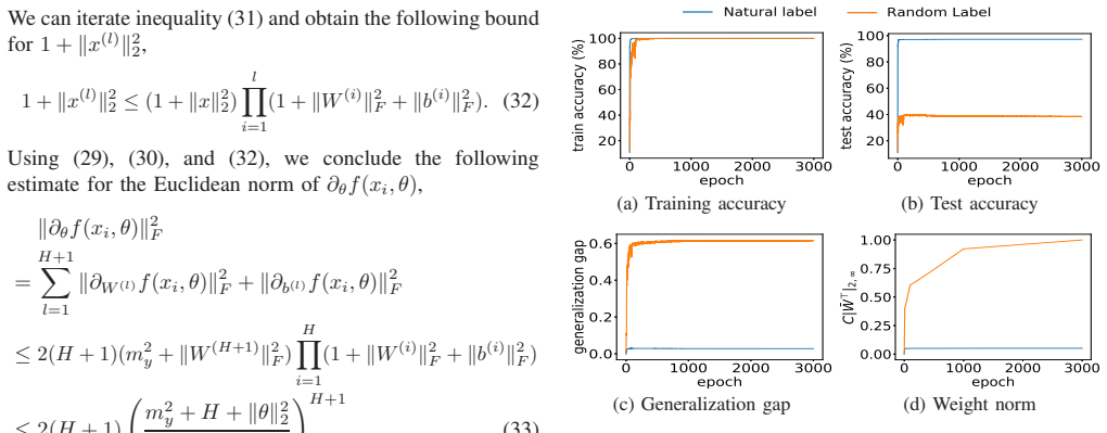
On the paper's own terms, the central discovery is a trainability guarantee for deep feedforward networks with $H \ge 2$ hidden layers: for any normalized dataset of $n$ input–output pairs, any convex Lipschitz loss, and any $\delta>0$, there is a network architecture with $d = O(((n + m_x H^2 + H^5 \log(Hn^2/\delta)) \log(Hn^2/\delta) + n m_y))$ parameters such that gradient descent with a per-coordinate learning rate reaches an $\epsilon$-global minimum of the empirical risk with probability at least $1-\delta$. The last hidden layer needs only $O(n)$ neurons, and earlier layers need only logarithmic widths. The matching lower bound says no architecture with fewer than $n m_y$ parameters can interpolate arbitrary labels without parameter norms growing like $n^{\beta}$, so the linear dependence on $n$ is optimal up to a logarithmic factor. The generalization result bounds expected 0–1 error by an empirical margin loss plus a term proportional to the output-layer weight norm divided by $\sqrt{n}$, and the experiments illustrate that this weight norm stays small for natural MNIST labels and grows for randomly corrupted labels.
Load-bearing premise
The proof needs every pair of distinct training inputs to end up with hidden representations separated by at least a fixed positive margin, and it chooses the network width dependent on that margin; since the theorem claims to cover all normalized datasets, including ones with arbitrarily close or identical inputs, the universal guarantee relies on a margin that the dataset class itself does not enforce.
Editorial extensions
If this is right
- Networks with parameter count linear in the number of training samples are provably trainable to global optimality by gradient descent, bringing the theory into the regime of real architectures such as PreActResNet18.
- The lower bound shows no trainability guarantee can do better than $\Omega(n m_y)$ parameters up to log factors, so the linear rate is the right target for future work.
- For shallow networks with $H=1$, the guarantee requires $O(n(m_x+m_y))$ parameters, so depth reduces the parameter cost when the input dimension is large.
- The generalization bound ties test error to the output-layer weight norm, giving a concrete mechanism by which the same network memorizes random labels with large norm but generalizes on natural labels with small norm.
Reading between the lines
- A testable extension suggested by the proof: the minimal last-layer width for guaranteed convergence should scale with the inverse of the smallest pairwise distance among training inputs, and an experiment could vary duplicate closeness and measure where gradient descent starts to fail.
- The full-rank feature matrix condition could be used as a data-dependent certificate of trainability: compute the smallest singular value of the hidden Gram matrix during training and predict convergence before it happens.
- The volume-based lower bound likely generalizes to any smooth parametric function class, yielding a general principle that fitting arbitrary labels to $n$ points with $d$ parameters forces weight norms to grow at least like $n^{\Omega((n m_y/d)-1)}$.
- Because the upper bound is proven for analytic activations that approximate ReLU, the theory may extend to ReLU by a limiting argument, but the margin condition would then need separate treatment for exactly zero hidden differences.
Signed reviews
Editorial analysis
A structured set of objections, weighed in public.
Referee Report
Summary. The paper defines a formal notion of probable trainability P_{n,H,δ}(d), and claims that for any depth H≥2 there is a network with Õ(n m_y + m_x H^2 + H^5) parameters such that gradient descent with per-coordinate learning rates reaches the functional global minimum L(f*) up to ε for every normalized dataset with probability at least 1−δ. The proof proceeds by fixing a random initialization, using concentration to show that the penultimate representations are well separated, proving that the random feature matrix M(w,b) has full row rank, and then solving the remaining convex last-layer problem. The paper also proves a lower bound showing that d ≥ n m_y is necessary, and gives a generalization bound together with experiments on several image datasets. A central gap is that the proof of Theorem 1 assumes a positive uniform separation margin γ that the dataset class S_n does not provide, and the learning-rate vector used in the proof has zero entries for all hidden layers; the advertised claim that all layers are optimized is therefore not derived as stated.
Significance. If the universal claim in Theorem 1 were correct, this would be a substantial advance: it would reduce the over-parameterization required for trainability from polynomial or 2^O(H) factors to Õ(n), prove a matching lower bound up to logarithms, and connect trainability to generalization. The paper also contains a clean random-feature reduction, a self-contained volume/Sard lower-bound argument, and informative experiments that support the qualitative predictions. However, the margin assumption in the proof and the last-layer-only update mean the main theorem as stated is not established; a corrected, possibly weaker theorem with a separation condition or a new uniform argument would still be valuable. The lower-bound and generalization sections appear largely sound.
major comments (3)
- [Section IV.A, equations (17)-(18) and Lemma 2] The proof introduces a quantity γ with p^(0)_ij = ||x_i−x_j||^2 ≥ γ and then asserts that, by considering C sufficiently large, equation (18) holds with a lower bound cγ that depends only on γ. In Definition 1 the architecture f, and hence C and all layer widths, must be fixed once for all datasets S ∈ S_n, but S_n contains datasets with arbitrarily close or even identical normalized inputs; no positive uniform γ exists over S_n. For such datasets the concentration error O(1/(cC)) in equation (17) cannot be made smaller than p^(H−1)_ij/2 for all pairs with a single fixed C; in the duplicate case p^(l)_ij = 0 for every l, so inequality (18) would read 0 > cγ. Consequently the hypothesis of Lemma 2 is not verified for all S, the step rank(M(w,b)) = n is not established, and the exact interpolation f(X,ψ(θ0,W*)) = f*(X) is not proved for the full dataset class. As written, the proof establishes Theorem 1 only for datasets with a uniform separation margin.
- [Section IV.A, after equation (21)] The proof sets η_i = 1/(c_z ζ) only for the output-layer coordinates and η_i = 0 otherwise, so the generated gradient-descent iterates leave every hidden-layer parameter at its random initial value. This means the advertised statement that gradient descent finds a global minimum of the non-convex optimization of all layers is not derived: the optimization actually performed is convex optimization of the final linear layer on fixed random features. The formal statement of Theorem 1 may be compatible with such an η, but the title, abstract, and introduction should either be restricted to the claim as proved or the proof must be extended to positive learning rates for the hidden layers.
- [Section IV.A, equations (17)-(18)] There is also a quantifier issue in the step leading to the full-rank event. For each fixed dataset S the rank-deficiency set may have measure zero, but Theorem 1 requires a 1−δ statement that holds for every S ∈ S_n, an uncountable family. The margin-based concentration argument is the only place where uniformity over S is provided, and it fails for the reason above; an additional covering/net argument, a restriction of S_n, or another uniform mechanism is needed to justify the universal claim.
minor comments (5)
- [Corollary 2] The quantity γ is used in the inequality p^(0)_ij = ||x_i−x_j||^2 ≥ γ before it is defined; the paper should state explicitly whether γ is a universal constant, a dataset-dependent margin, or a parameter of the proof, and it should specify its role in the quantifier structure of Theorem 1.
- [Section IV.A, equation (18)] The remark that the constant cγ depends only on γ is insufficient because p^(H−1)_ij also depends on the activation function σ and on the entire collection of inputs; the text should provide the precise dependence so that the required size of C relative to the data can be checked.
- [End of proof of Theorem 1] The sentence '... ≤ cθ for some constant in ε>0' is garbled; according to Definition 1, cθ must be chosen before ε, and the proof should be rewritten to make clear that cθ is independent of ε.
- [Appendix, proof of Proposition 1] With the choice δ'_k = 6δ'/(π^2 k^2), the union-bound logarithm in inequality (35) should be ln(π^2 k^2/(6δ'))/(2n), not ln(π^2⌈ς‖W^T‖_{2,∞}⌉^2/δ')/(2n); the displayed bound is still valid up to absolute constants, but the derivation as written does not match the displayed formula.
- [Figure 2(d)] The axis label is rendered as 'C| /uni0304W /uni22A4|2̄ ∞' and the caption refers to 'C‖W^T‖_{2,∞}' without defining C; the normalization constant should be defined for the reader.
Circularity Check
No significant circularity: the trainability proof is a genuine reduction to random-feature interpolation and last-layer convex optimization, and the generalization bound is an external Rademacher argument.
full rationale
I walked the derivation chain of Theorem 1. The proof first establishes concentration of the hidden representations (Corollary 2), then proves that the random feature matrix M has rank n for m_H >= n under a separation condition (Lemma 2), and finally trains only the last layer with gradient descent on a convex objective while holding the earlier layers at their random initialization. Interpolating the arbitrary global minimizer f* on the n training points via rank(M)=n is a substantive reduction, not an assumption of the conclusion; the lower bound L(f*) <= J(theta) makes the argument valid rather than circular wherever the separation hypothesis is available. No parameter is fitted to a subset of the data and then renamed a prediction: the widths are chosen as functions of n, H, and delta only, and the constant C is introduced as an over-parameterization scale, not as a data-fitted value. Theorem 2 is an independent volume/Jacobian lower bound, and Proposition 1 applies the external Rademacher bound of Koltchinskii and Panchenko; the self-citations [22] and [23] appear only in the closing contrast paragraph and are not load-bearing. The margin concern raised in Section IV.A (equations (17)-(18)) is a genuine proof gap but not a circularity: for duplicate inputs p_ij^(0)=0 and hence p_ij^(H-1)=0, so the inequality '> c_gamma' in (18) cannot hold for any C, and Lemma 2's rank-n conclusion is not available for all datasets in S_n. This means the proof as written establishes trainability for gamma-separated datasets, not for the full class S_n; however, this is a missing hypothesis or a failed universal quantification, not a case where the theorem's output is equivalent to its input by construction. Consequently the circularity score is 0.
Assumptions & free parameters
assumptions (6)
- domain assumption The loss criterion q -> ell(q, y_i) is differentiable, convex, nonnegative, and has a zeta-Lipschitz gradient (Assumption 1).
- domain assumption The activation function sigma is real analytic, monotonically increasing, 1-Lipschitz, and has one-sided limits (Assumption 2).
- domain assumption Training inputs are normalized as ||x_i||^2 = 1 and labels satisfy y_i in [-1,1]^{m_y} (definition of S_n).
- standard math The zero set of a nonzero real analytic function has Lebesgue measure zero (Mityagin [20]).
- standard math Sard's theorem and the rank theorem for smooth or analytic maps, used to bound the volume of the image of the parameter-to-output map.
- domain assumption For each dataset and loss functional, a global minimizer f* of the functional L exists (part of the definition of L^zeta_S).
Cite this review
Pith. "Pith review of Gradient Descent Finds Global Minima for Generalizable Deep Neural Networks of Practical Sizes." pith.science (2026). https://pith.science/paper/A5GNHRV5
@misc{pith2026190802419,
  author       = {Pith},
  title        = {Pith review of: Gradient Descent Finds Global Minima for Generalizable Deep Neural Networks of Practical Sizes},
  year         = {2026},
  howpublished = {\url{https://pith.science/paper/A5GNHRV5}},
  note         = {Machine review of arXiv:1908.02419}
}
read the original abstract
In this paper, we theoretically prove that gradient descent can find a global minimum of non-convex optimization of all layers for nonlinear deep neural networks of sizes commonly encountered in practice. The theory developed in this paper only requires the practical degrees of over-parameterization unlike previous theories. Our theory only requires the number of trainable parameters to increase linearly as the number of training samples increases. This allows the size of the deep neural networks to be consistent with practice and to be several orders of magnitude smaller than that required by the previous theories. Moreover, we prove that the linear increase of the size of the network is the optimal rate and that it cannot be improved, except by a logarithmic factor. Furthermore, deep neural networks with the trainability guarantee are shown to generalize well to unseen test samples with a natural dataset but not a random dataset.
Figures

Reference graph
Works this paper leans on
-
[1]
On the capabilities of multilayer perceptro ns,
E. B. Baum, “On the capabilities of multilayer perceptro ns,” J. Complexity, vol. 4, no. 3, pp. 193–215, 1988. [Online]. Available: https://doi.org/10.1016/0885-064X(88)90020-9
-
[2]
T. M. Cover, “Geometrical and statistical properties of systems of linear inequalities with applications in pattern recognit ion,” IEEE Trans. Electronic Computers , vol. 14, no. 3, pp. 326–334, 1965. [Online]. Available: https://doi.org/10.1109/PGEC.196 5.264137
-
[3]
Learning capability and storage capacity of t wo- hidden-layer feedforward networks,
G. Huang, “Learning capability and storage capacity of t wo- hidden-layer feedforward networks,” IEEE Trans. Neural Networks , vol. 14, no. 2, pp. 274–281, 2003. [Online]. Available: https://doi.org/10.1109/TNN.2003.809401
arXiv 2003
-
[4]
Bounds on the number of hidden neur ons in multilayer perceptrons,
S. Huang and Y . Huang, “Bounds on the number of hidden neur ons in multilayer perceptrons,” IEEE Trans. Neural Networks , vol. 2, no. 1, pp. 47–55, 1991. [Online]. Available: https://doi.org/10 .1109/72.80290
work page 1991
-
[5]
G. Huang and H. A. Babri, “Upper bounds on the number of hid den neurons in feedforward networks with arbitrary bounded non linear activation functions,” IEEE Trans. Neural Networks , vol. 9, no. 1, pp. 224–229, 1998. [Online]. Available: https://doi.org/10. 1109/72.655045
work page 1998
-
[6]
The lower bound of the capacity for a neural network with multiple hidden layers,
M. Y amasaki, “The lower bound of the capacity for a neural network with multiple hidden layers,” in International Conference on Artificial Neural Networks . Springer, 1993, pp. 546–549
work page 1993
-
[7]
Small relu networks are powerful memorizers: a tight analysis of memorization capacity,
C. Y un, S. Sar, and A. Jadbabaie, “Small relu networks are powerful memorizers: a tight analysis of memorization capacity,” arXiv preprint, arXiv:1810.07770, 2018
arXiv 2018
-
[8]
Identity matters in deep learning,
M. Hardt and T. Ma, “Identity matters in deep learning,” i n Interna- tional Conference on Learning Representations , 2017
work page 2017
Show all 24 references
-
[9]
Optimization landscape and expre ssivity of deep cnns,
Q. Nguyen and M. Hein, “Optimization landscape and expre ssivity of deep cnns,” in Proceedings of the 35th International Conference on Machine Learning, ICML 2018, Stockholmsm¨ assan, Stockh olm, Sweden, July 10-15, 2018 , 2018, pp. 3727–3736. [Online]. Available: http://proce...
2018
-
[10]
Hardness results for neu ral network approximation problems,
P . Bartlett and S. Ben-David, “Hardness results for neu ral network approximation problems,” in European Conference on Computational Learning Theory . Springer, 1999, pp. 50–62
1999
-
[11]
Training a 3-node neural netwo rk is np-complete,
A. Blum and R. L. Rivest, “Training a 3-node neural netwo rk is np-complete,” in Advances in neural information processing systems , 1989, pp. 494–501
1989
-
[12]
On the comp utational efficiency of training neural networks,
R. Livni, S. Shalev-Shwartz, and O. Shamir, “On the comp utational efficiency of training neural networks,” in Advances in Neural Infor- mation Processing Systems , 2014, pp. 855–863
2014
-
[13]
Learning overparameterized neural networks via stochastic gradient descent on structured data,
Y . Li and Y . Liang, “Learning overparameterized neural networks via stochastic gradient descent on structured data,” in Advances in Neural Information Processing Systems , 2018, pp. 8157–8166
2018
-
[14]
Gradient desc ent provably optimizes over-parameterized neural networks,
S. S. Du, X. Zhai, B. Poczos, and A. Singh, “Gradient desc ent provably optimizes over-parameterized neural networks,” In ICLR, arXiv:1810.02054, 2018
2018 arXiv
-
[15]
Quadratic suffices for over-parame trization via matrix chernoff bound,
Z. Song and X. Y ang, “Quadratic suffices for over-parame trization via matrix chernoff bound,” arXiv preprint arXiv:1906.03593 , 2019
1906 arXiv
-
[16]
A convergence theory f or deep learning via over-parameterization,
Z. Allen-Zhu, Y . Li, and Z. Song, “A convergence theory f or deep learning via over-parameterization,” In ICML, arXiv:1811.03962 , 2018
2018 arXiv
-
[17]
Gradi- ent descent finds global minima of deep neural networks,
S. S. Du, J. D. Lee, H. Li, L. Wang, and X. Zhai, “Gradi- ent descent finds global minima of deep neural networks,” ICML, arXiv:1811.03804, 2018
2018 arXiv
-
[18]
Stochastic gradient d escent optimizes over-parameterized deep relu networks,
D. Zou, Y . Cao, D. Zhou, and Q. Gu, “Stochastic gradient d escent optimizes over-parameterized deep relu networks,” arXiv preprint arXiv:1811.08888, 2018
2018 arXiv
-
[19]
An improved analysis of training over-parameterized deep neural networks,
D. Zou and Q. Gu, “An improved analysis of training over-parameterized deep neural networks,” arXiv preprint arXiv:1906.04688, 2019
1906 arXiv
-
[20]
The zero set of a real analytic function,
B. Mityagin, “The zero set of a real analytic function,” arXiv preprint arXiv:1512.07276, 2015
2015 arXiv
-
[21]
Gradien t-based learning applied to document recognition,
Y . LeCun, L. Bottou, Y . Bengio, and P . Haffner, “Gradien t-based learning applied to document recognition,” Proceedings of the IEEE , vol. 86, no. 11, pp. 2278–2324, 1998
1998
-
[22]
Depth with nonlinearity cr eates no bad local minima in ResNets,
K. Kawaguchi and Y . Bengio, “Depth with nonlinearity cr eates no bad local minima in ResNets,” Neural Networks , vol. 118, pp. 167–174, 2019. [Online]. Available: arXiv:1810.09038
2019 arXiv
-
[23]
Every loca l minimum value is the global minimum value of induced model in non-con vex machine learning,
K. Kawaguchi, J. Huang, and L. P . Kaelbling, “Every loca l minimum value is the global minimum value of induced model in non-con vex machine learning,” Neural Computation, to appear , 2019. [Online]. Available: arXiv:1904.03673
2019 arXiv
-
[24]
Empirical margin di stributions and bounding the generalization error of combined classifiers,
V . Koltchinskii and D. Panchenko, “Empirical margin di stributions and bounding the generalization error of combined classifiers, ” Annals of Statistics, pp. 1–50, 2002
2002
Reviewed August 14, 2026 · model on record in the stance chip above.
Discussion (0). Continue with ORCID to comment.