Gradient Descent as a Perceptron Algorithm: Understanding Dynamics and Implicit Acceleration
Pith reviewed 2026-05-22 12:06 UTC · model grok-4.3
The pith
Gradient descent on nonlinear models with logistic loss reduces to generalized perceptron updates.
A machine-rendered reading of the paper's core claim, the machinery that carries it, and where it could break.
Core claim
We analyze nonlinear models with the logistic loss and show that the steps of GD reduce to those of generalized perceptron algorithms, providing a new perspective on the dynamics. This reduction yields significantly simpler algorithmic steps, which we analyze using classical linear algebra tools. Using these tools, we demonstrate on a minimalistic example that the nonlinearity in a two-layer model can provably yield a faster iteration complexity Õ(√d) compared to Ω(d) achieved by linear models, where d is the number of features. This helps explain the optimization dynamics and the implicit acceleration phenomenon observed in neural networks.
What carries the argument
The exact reduction that rewrites each gradient descent step as a generalized perceptron update on the two-layer nonlinear model with logistic loss.
If this is right
- Dynamics of convergence, trajectories, and oscillations become analyzable with elementary linear algebra once the perceptron equivalence is used.
- Nonlinearity in the two-layer case produces iteration complexity scaling as Õ(√d) while linear models require Ω(d) steps.
- Implicit acceleration observed during neural network training can be traced to the perceptron-like behavior induced by the nonlinear layers.
- Oscillations in function values during training follow directly from known properties of generalized perceptron algorithms.
Where Pith is reading between the lines
- The same reduction technique could be attempted on deeper networks or with different nonlinear activations to see whether similar acceleration appears.
- New optimization procedures might be constructed by directly simulating the perceptron updates instead of computing gradients.
- Empirical checks on high-dimensional datasets could reveal whether the square-root scaling persists beyond the minimal example.
- The perspective links modern neural optimization to classical linear classifiers and may illuminate other implicit-bias effects.
Load-bearing premise
The claimed reduction of every gradient descent step to a perceptron update and the resulting complexity comparison are derived only for a minimal two-layer nonlinear model.
What would settle it
Running gradient descent on the two-layer logistic model and checking whether the exact sequence of parameter changes matches the perceptron update rule would directly test the reduction.
Figures






read the original abstract
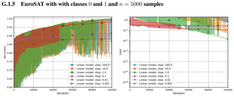
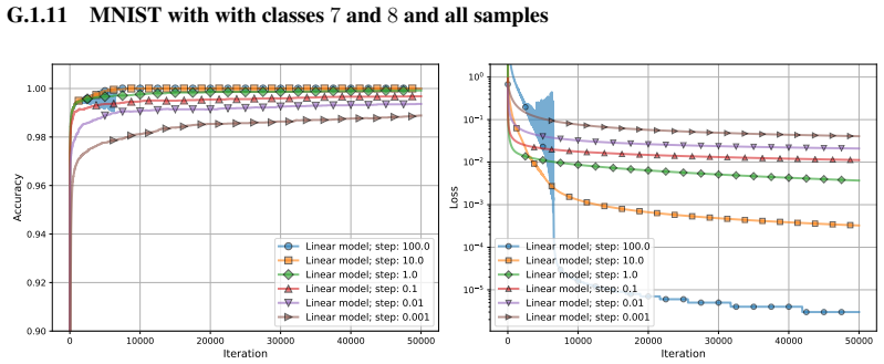
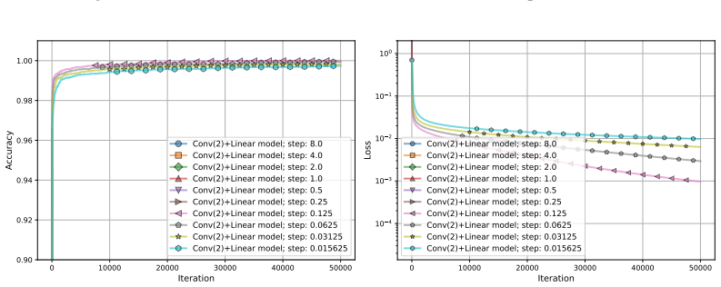
Even for the gradient descent (GD) method applied to neural network training, understanding its optimization dynamics, including convergence rate, iterate trajectories, function value oscillations, and especially its implicit acceleration, remains a challenging problem. We analyze nonlinear models with the logistic loss and show that the steps of GD reduce to those of generalized perceptron algorithms (Rosenblatt, 1958), providing a new perspective on the dynamics. This reduction yields significantly simpler algorithmic steps, which we analyze using classical linear algebra tools. Using these tools, we demonstrate on a minimalistic example that the nonlinearity in a two-layer model can provably yield a faster iteration complexity $\tilde{O}(\sqrt{d})$ compared to $\Omega(d)$ achieved by linear models, where $d$ is the number of features. This helps explain the optimization dynamics and the implicit acceleration phenomenon observed in neural networks. The theoretical results are supported by extensive numerical experiments. We believe that this alternative view will further advance research on the optimization of neural networks.
Editorial analysis
A structured set of objections, weighed in public.
Referee Report
Summary. The paper argues that gradient descent applied to nonlinear models with the logistic loss can be exactly reduced to generalized perceptron algorithm steps. This reduction simplifies the analysis of optimization dynamics using classical linear algebra. On a minimal two-layer nonlinear model, they show a provable iteration complexity of ~O(sqrt(d)) versus Omega(d) for linear models, which they suggest explains implicit acceleration in neural networks. The theoretical findings are corroborated by numerical experiments.
Significance. Should the reduction hold and extend to more general settings, this work would provide a fresh perspective on why gradient descent exhibits certain behaviors in neural network training, particularly the role of nonlinearity in achieving faster convergence. The complexity separation in the toy model is a concrete demonstration of this advantage, though its relevance to practical deep networks hinges on broader applicability.
major comments (3)
- [Abstract and §3] Abstract and §3: The assertion that GD steps reduce to generalized perceptron updates for 'nonlinear models' is supported by derivation only in the minimalistic two-layer logistic loss setting; the algebraic cancellation shown does not immediately generalize to deeper architectures or other activations, which is critical for the explanation of implicit acceleration in general neural networks.
- [§4] §4, complexity bound derivation: The ~O(sqrt(d)) complexity is proven for the two-layer example, but the manuscript does not provide a corresponding analysis or bound for linear models within the same perceptron reduction framework to rigorously establish the separation; the Omega(d) is cited from classical results without integration.
- [§5] §5, Experiments: The numerical experiments validate the theory on the minimal example, but lack ablations on slightly deeper models to test if the reduction and acceleration persist, leaving the extrapolation to general NNs untested.
minor comments (3)
- [Introduction] The citation to Rosenblatt (1958) should be expanded with full bibliographic details for completeness.
- [Figures] The plot labels and legends in the figures could be made larger for better readability in the final version.
- [Notation] Some symbols like the generalized perceptron update rule are introduced without sufficient preliminary definition before use in the main theorems.
Simulated Author's Rebuttal
We thank the referee for their constructive comments, which help clarify the scope of our results. We address each major comment point by point below, with revisions where appropriate to improve precision without altering the core contributions.
read point-by-point responses
-
Referee: [Abstract and §3] The assertion that GD steps reduce to generalized perceptron updates for 'nonlinear models' is supported by derivation only in the minimalistic two-layer logistic loss setting; the algebraic cancellation shown does not immediately generalize to deeper architectures or other activations.
Authors: We agree that the exact reduction via algebraic cancellation is derived for the two-layer model. The manuscript presents this as a minimalistic example to illustrate the perspective on implicit acceleration. We will revise the abstract and Section 3 to explicitly qualify the claims as applying to this setting and to state that extensions to deeper architectures or other activations are left as future work. revision: yes
-
Referee: [§4] The ~O(sqrt(d)) complexity is proven for the two-layer example, but the manuscript does not provide a corresponding analysis or bound for linear models within the same perceptron reduction framework to rigorously establish the separation; the Omega(d) is cited from classical results without integration.
Authors: The linear case reduces precisely to the standard perceptron algorithm under the same framework, so the classical Ω(d) bound applies directly. To integrate the comparison rigorously, we will add a short subsection in Section 4 that recalls the classical perceptron bound using the linear algebra tools developed for the nonlinear analysis, thereby establishing the separation within our unified view. revision: yes
-
Referee: [§5] The numerical experiments validate the theory on the minimal example, but lack ablations on slightly deeper models to test if the reduction and acceleration persist, leaving the extrapolation to general NNs untested.
Authors: Our experiments are tailored to validate the theory on the minimal two-layer model. Adding ablations on deeper models would require new theoretical approximations for the reduction, which exceeds the current scope. We will expand the discussion in Section 5 to explicitly note this limitation and identify deeper-model testing as future work; this constitutes a partial revision. revision: partial
- Generalization of the perceptron reduction and complexity separation to arbitrary deep architectures or activations.
Circularity Check
No significant circularity detected; derivation relies on algebraic reduction and external linear-algebra analysis
full rationale
The paper derives an equivalence between GD steps and generalized perceptron updates directly from the logistic loss on a two-layer nonlinear model, then applies classical linear-algebra tools to obtain the O(sqrt(d)) vs Omega(d) complexity separation. This chain is presented as explicit algebraic manipulation rather than a parameter fit, self-referential definition, or load-bearing self-citation. The minimalistic example is used to demonstrate the nonlinearity benefit without assuming the target implicit-acceleration phenomenon as an input. No steps reduce by construction to the paper's own fitted values or prior self-citations.
Axiom & Free-Parameter Ledger
axioms (1)
- domain assumption Gradient-descent iterates on the logistic loss for the nonlinear models under study are exactly equivalent to updates of a generalized perceptron algorithm.
Reference graph
Works this paper leans on
-
[1]
Risk and parameter convergence of logistic regression
PMLR. Ji, Z. and Telgarsky, M. (2018). Risk and parameter convergence of logistic regression.arXiv preprint arXiv:1803.07300. Kreisler, I., Nacson, M. S., Soudry, D., and Carmon, Y . (2023). Gradient descent monotonically decreases the sharpness of gradient flow solutions in scalar networks and beyond. InInternational Conference on Machine Learning, pages...
work page internal anchor Pith review Pith/arXiv arXiv 2018
-
[2]
Ifa= 0,thenAis the zero matrix withd+ 2zero eigenvalues
-
[3]
If a̸= 0 and a=Pa, then A has two non-zero eigenvalues √ 2∥a∥ and − √ 2∥a∥ with the corresponding eigenvectorsv 1 = ∥a∥ ∥a∥ √ 2a⊤ ⊤ andv 2 = − ∥a∥ − ∥a∥ √ 2a⊤ ⊤
-
[4]
If a̸= 0 and a=−Pa, then A has two non-zero eigenvalues √ 2∥a∥ and − √ 2∥a∥ with the corresponding eigenvectorsv 1 = ∥a∥ − ∥a∥ √ 2a⊤ ⊤ andv 2 = − ∥a∥ ∥a∥ √ 2a⊤ ⊤
-
[5]
If a̸= 0, a̸=Pa, and a̸=−Pa, then A has four non-zero eigenvalues q ∥a∥2 +a ⊤Pa, − q ∥a∥2 +a ⊤Pa, q ∥a∥2 −a ⊤Pa,− q ∥a∥2 −a ⊤Pawith the corresponding eigenvectors v1 = ¯a+,P ¯a+,P (a+Pa) ⊤ ⊤ , v2 = −¯a+,P −¯a+,P (a+Pa) ⊤ ⊤ , v3 = ¯a−,P −¯a−,P (a−Pa) ⊤ ⊤ ,andv 4 = −¯a−,P ¯a−,P (a−Pa) ⊤ ⊤ , where¯a+,P := q ∥a∥2 +a ⊤Paand¯a−,P := q ∥a∥2 −a ⊤Pa. 5.∥a∥ ≤ ∥A∥ ≤...
-
[6]
A1 has two non-zero eigenvalues λ1 and −λ1 with the corresponding eigenvectors v1,+ and v1,−, whereλ 1 := √ 2d
-
[7]
A2 has four non-zero eigenvalues λ2,−λ 2, µ,−µ with the corresponding eigenvectors v2,+, v2,−, vµ,+,andv µ,−,whereλ 2 := p (2 +µ) 2 + 2(d−2). 3.v µ,+, vµ,− ∈ker(A 1). Proof. The first and second result are simple corollaries of Proposition 4.1. The third result follows from thatv µ,+ andv µ,− are propositional to [−µ µ µ−µ0. . .0 ]⊤ , [µ−µ µ−µ0. . .0 ]⊤ ....
work page 2027
-
[9]
⟨θt, vµ,−⟩2 + 4∥ξ t∥ ∥θt∥+∥ξ t∥2 1 +γ 2λ2 2 , 30 where we have arranged terms. Substituting to (42), ∥θt+1∥2 ≤(1 +s) " (1 +γ 2λ2 2)(⟨θt, v2,+⟩2 +⟨θ t, v2,−⟩2) + 2γλ2 − 2γλ2 1 +γ 2λ2 2 (⟨θt, v2,+⟩2 +⟨θ t, v2,−⟩2)− µ(1 +γµ) 2 λ2(1 +γ 2λ2
-
[10]
⟨θt, vµ,+⟩2 + µ(1−γµ) 2 λ2(1 +γ 2λ2
-
[11]
⟨θt, vµ,−⟩2 + 2γλ2 4∥ξ t∥ ∥θt∥+∥ξ t∥2 1 +γ 2λ2 2 ! + (1 +γµ) 2 ⟨θt, vµ,+⟩2 + (1−γµ) 2 ⟨θt, vµ,−⟩2 + d−2X j=1 ⟨θt, v2,j⟩2 # + (1 +s −1)∥ξ t∥2 . Since0≤γ≤ 1 λ2 and0≤γ≤ 1 µ , ∥θt+1∥2 ≤(1 +s) " ⟨θt, v2,+⟩2 +⟨θ t, v2,−⟩2 + (1 +γµ) 2 (1−γµ)⟨θ t, vµ,+⟩2 + (1−γµ) 2 (1 + 2γµ)⟨θ t, vµ,−⟩2 + d−2X j=1 ⟨θt, v2,j⟩2 # + (1 +s −1)∥ξ t∥2 + (1 +s)2γλ 2 4∥ξ t∥ ∥θt∥+∥ξ t∥2 ≤...
work page 2017
discussion (0)
Sign in with ORCID, Apple, or X to comment. Anyone can read and Pith papers without signing in.