REVIEW 2 major objections 4 minor 58 references
The paper claims that in a matrix model of two-color two-flavor QCD, tuning baryon, isospin, and chiral chemical potentials drives a web of first-order quantum phase transitions, with several phases having spin-1 ground states that spontane
Reviewed by Pith at T0; open to challenge. T0 means a machine referee read the full paper against a public rubric. the ladder, T0–T4 →
T0 review · deepseek-v4-flash
2026-08-01 19:58 UTC pith:ACKNWM5K
load-bearing objection Genuinely new phase diagram for matrix-QCD2,2 at large chemical potentials, honestly presented; the main caveat is that the ground-state search is restricted to J=0 and J=1 by assertion, not by evidence. the 2 major comments →
Quantum phases at high chemical potential in 2-flavor matrix-QC₂D
The pith
A machine-rendered reading of the paper's core claim, the machinery that carries it, and where it could break.
Core claim
The central claim is that the matrix model of gauge field theory with two colors and two flavors, when projected to its color-singlet sector and restricted to large chemical potentials, has a ground-state phase diagram organized by level crossings. In the limit where the baryon and chiral chemical potentials are both large while their difference stays finite, the low-energy Hilbert space reduces to pure antiquark (or quark) states, and diagonalizing the effective Hamiltonian reveals four level crossings in the isospin-0 sector, two in the isospin-±1 sector, and none in the isospin-±2 sector. When the isospin chemical potential is switched on, crossings between different isospin sectors produ
What carries the argument
The machinery is the variational diagonalization of the matrix-model Hamiltonian in a truncated harmonic-oscillator basis for the three-by-three glue matrix, with the number of oscillator quanta cut off around 16 (convergence checked against 18). In the large-chemical-potential limits, the effective Hamiltonian becomes a single-particle problem on a finite fermionic sector (up to four antiquarks or quarks) coupled to the glue, and the ground state is found by comparing the lowest color-singlet energies in sectors labelled by isospin I and baryon number B. Level crossings between these sectors as functions of the potential differences define the first-order quantum phase transitions. The spin
Load-bearing premise
The load-bearing premise is the variational truncation of the infinite-dimensional glue Hilbert space: all phase boundaries and spin fractions come from diagonalizing the Hamiltonian with a harmonic-oscillator cutoff of roughly 16 quanta, and the ground-state search is restricted to spin-0 and spin-1 sectors; if a low-lying state outside this truncation or in a higher-spin sector exists, the phase diagram could shift.
What would settle it
A concrete falsifier would be a variational diagonalization with a substantially larger basis (e.g., Nb=24 or using a different basis) that shows the level-crossing positions and spin fractions changing beyond numerical error, or a lattice simulation of two-color QCD at large baryon/isospin/chiral chemical potentials that fails to find a spin-1 di-(anti-)quark ground state breaking rotational symmetry.
If this is right
- If the phase web is correct, two-color QCD at large baryon and isospin chemical potentials should show first-order transitions where baryon number and isospin jump discontinuously.
- The spin-1 phases provide a concrete zero-momentum signature — spontaneous breaking of rotational symmetry — that could be searched for in lattice simulations of two-color QCD, which are free of the sign problem.
- The spin fractions give quantitative predictions for how much of the angular momentum in a LOFF-like ground state resides in the quark pairs, a quantity that could be compared with effective field theory.
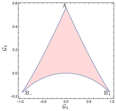
- The phases I−2 (at strong coupling) and massless phase IV exhibit a diverging expectation value of the glue-field squared and Binder cumulants at the tip of the allowed region, indicating a possible non-regular representation of the Weyl algebra; this is a new strong-coupling phenomenon to be understood.
- The existence of a web of phases spanning intermediate and strong coupling suggests the matrix model can be used as a controlled setting to map the dense-matter phase structure of QCD-like theories.
Where Pith is reading between the lines
- If the matrix-model result survives in full two-color QCD, the LOFF phases predicted by effective field theory would be observable in lattice simulations at finite isospin or chiral chemical potential, since those simulations are not obstructed by the sign problem.
- The spin-1 diquark phases may be the two-color analogue of spin-1 (or vector) condensation in three-color dense QCD, potentially relevant for neutron-star matter; however, the matrix model is only a zero-momentum toy model, so this extrapolation is speculative.
- The strong sensitivity of certain observables (the glue expectation and the fourth-order cumulant) to the oscillator cutoff in phases I−2 and IV might be a numerical artifact of the truncation; a larger-basis or non-Gaussian variational calculation could confirm whether the divergence is physical or an artifact.
- The paper restricts the ground-state search to spin-0 and spin-1 sectors; a systematic scan including spin-2 or higher could reveal additional phases that would modify the phase diagram.
Editorial analysis
A structured set of objections, weighed in public.
Referee Report
Summary. The paper studies the SU(2) two-flavor matrix model (‘matrix-QCD_{2,2}’) at large baryon, isospin and/or chiral chemical potentials. The authors derive effective Hamiltonians in the limits μ_B→∞, c→∞ (Section 2.1 and Eq. (2.6)), and μ_B→∞, μ_I→∞ (Eq. (2.8)), then diagonalize the color-singlet sector variationally with a harmonic-oscillator cutoff N_b. The central results are the phase diagrams in the Δ–|μ_I| plane (Fig. 7, Table 1) and in the c–|μ_BI| plane (Fig. 13, Table 3), in which the ground state is labelled by baryon number B and isospin I. Several phases (II_B in Section 3.1 and V_± in Section 3.2) are claimed to be spin-1 triplets that spontaneously break rotational symmetry and are interpreted as LOFF-like analogues of the diquark-condensate states predicted by Splittorff–Son–Stephanov [32]. The paper also computes Binder-like observables G_3, G_4 and Φ, and fermionic spin fractions f_B and F(ν,m).
Significance. If the reported ground states are correct, the paper provides a concrete microscopic realization of LOFF-like spin-1 phases in a strongly coupled two-color gauge model, going beyond effective field theory and complementing lattice studies. The effective large-chemical-potential reductions are transparent, the Hamiltonian is well defined, and the comparison with [32] is used as a consistency check rather than an input — I see no circularity in the main argument. However, the central numerical claim rests on (i) a variational truncation of the infinite-dimensional glue Hilbert space and (ii) a restriction of the ground-state search to spin-0 and spin-1 sectors. Neither of these is supported to the standard required for a phase diagram, and the paper provides no code, data, or error estimates. The significance is therefore conditional on closing those gaps.
major comments (2)
- [§3.1 and §3.2 (spin-sector restriction)] The ground-state search is restricted by assertion to J=0 and J=1: Section 3.1 says states in other sectors ‘are not relevant for this discussion as their energies are significantly higher,’ and Section 3.2 states that the lightest ℓ=0, ±2 states are spin-0 and ℓ=±1 is spin-1, without showing higher-J energies. Since [H,J_i]=0, sectors of different J are decoupled and the true ground state must be obtained by comparing all integer-J sectors. J≥2 states are kinematically allowed (the glue Hilbert space contains arbitrary L, and four quarks/antiquarks can carry S=2). If any J≥2 color-singlet state lies below the reported J=0/1 states in any region of (ν,Δ,μ_I,m,μ_BI), then Tables 1 and 3, the phase diagrams, and the central LOFF-like spin-1 claim all change. Please provide a systematic scan over J, or an analytic bound showing that higher-J sectors are separated by a gap, for each phase di
- [§3.1, Eqs. (3.8)–(3.9), (3.17)–(3.19), and Table 2] The paper states that energies converge for N_b=16 and 18, but the observables G_4 and Φ used to characterize phases I_-2 and IV are strongly N_b-dependent and are extrapolated using multi-parameter fits of ad hoc functional forms. For example, G_4[I_-2] at ν=0 is fitted as a tanh(b N_b−d)+k/N_b^α (Eq. (3.8)) with five parameters; this is the sole basis for the claim that (G_3,G_4) lies at the tip A. Similarly, the massless phase IV and V_± extrapolations in Eqs. (3.17)–(3.19) have no theoretical justification and no error bars. The spin fractions f_B and F(ν,m), which are central to the LOFF interpretation, are computed from the variational coefficients c_sℓ but their convergence with N_b is not shown. Please demonstrate that the extrapolations are stable under changes of N_b and fit form, and provide error estimates or code/data for reproducibility. Without this, the N_b→∞ entries in T
minor comments (4)
- [General] The numerical implementation is described only in words. For a paper whose central results are numerical, deposition of the diagonalization code and the parameters used (N_b, basis truncation, number of states retained per J sector) would substantially aid reproducibility.
- [§3.1, Figure 6 caption] The caption states μ_I = 1.5, but the text describing the figure does not specify the same value; please ensure the figure, caption, and text use consistent units and parameter values.
- [Table 2 and Table 4] The tables label columns as ‘N_b→∞ limit,’ but only some entries are obtained by explicit N_b extrapolation; other entries are stated to converge at N_b≈16. Please distinguish converged values from extrapolated values, e.g., with a footnote.
- [§3.1.1, Eq. (3.14)] The notation (s,ℓ) in Eq. (3.14) is clear, but the text preceding it says the glue states have spin 0, 1 or 2, while the sum only includes (s,ℓ) with s=0,1. It would help to state explicitly that fermionic states with odd number of quarks are excluded by color-singletness, so no s=2 fermionic term appears.
Circularity Check
No significant circularity — the phase structure is obtained by direct variational diagonalization; self-citations are methodological and the Splittorff-Son-Stephanov comparison is a consistency check, not an input.
full rationale
The central derivation is self-contained. The Hamiltonian is stated in Eqs. (2.2)-(2.3), and the effective Hamiltonians at large chemical potentials, Eqs. (2.6)-(2.8), follow from explicit large-μ projections onto sectors with fixed quark/antiquark numbers; they do not presuppose any particular phase. The phase diagrams in Figs. 7 and 13, and Tables 1 and 3, are constructed from level crossings among energy eigenvalues obtained by numerical diagonalization of these Hamiltonians. The spin-1 LOFF-like phases are identified from the computed ground-state quantum numbers and from the response of the degenerate triplet to the perturbation in Eq. (3.10); this is a direct calculation, not a restatement of an input. The comparison with Splittorff-Son-Stephanov [32] is explicitly presented as consistency ('These results are consistent with older effective field theory predictions') and the paper does not import [32]'s phase boundaries or condensate forms. Self-citations [51,52] supply the variational numerical strategy, definitions of Binder cumulants, and interpretive analogies (tip-A phase, Weyl-algebra divergence); none of these is used to force the phase boundaries or the existence of the spin-1 ground states. The G4 and Φ fits, Eqs. (3.8)-(3.9) and (3.17)-(3.19), are post-hoc descriptions of numerical data used to estimate the N_b→∞ limit; they are not used to define which phase is the ground state, so they do not make a prediction equivalent to its input. The restriction to J=0 and J=1 sectors and possible missing higher-spin states is a completeness/correctness assumption, not a circular reduction: it does not assume the conclusion, though it does limit the confidence in the global phase diagram.
Axiom & Free-Parameter Ledger
free parameters (5)
- G4 fit parameters for phase I_-2 at nu=0 =
a~0.5615~9/16, b~0.1065, d~0.338, k~32.53, alpha~5/2
- G4 fit parameters for phases IV and V+- at m=0, nu=0 =
IV: a~9/16, b~0.103, d~0.294, k~15.19, alpha~2.2; V+-: a~0.43, b~0.119, d~-0.571, k~-2.17, alpha~1.9
- Phi extrapolation parameters =
Phi ~ 3.58 + 0.44 N_b for I_-2/IV; V+- fit in Eq. (3.19)
- Variational coefficients c_sl in the spin decomposition =
not listed; determined by numerical ground-state wavefunction
- Bosonic harmonic-oscillator cutoff N_b =
~16, checked against 18
axioms (6)
- domain assumption Matrix model construction (Maurer-Cartan pullback to S^3 and zero-momentum projection) approximates low-energy QC2D
- domain assumption In the mu_B -> infinity, c -> infinity limit with finite Delta, the mass term is negligible and low-energy states contain only antiquarks with 0 <= N_d <= 4
- domain assumption The ground state lies in the spin-0 and spin-1 color-singlet sectors
- domain assumption Variational truncation at N_b ~ 16 converges to the exact low-lying spectrum
- standard math Degenerate perturbation theory with an epsilon*J perturbation diagnoses spontaneous SO(3) breaking in a finite quantum system
- standard math Physical states are color singlets, imposed by the Gauss-law constraint
read the original abstract
We investigate the matrix model of two-color two-flavor QCD (matrix-QCD$_{2,2}$) in regimes with large baryon ($\mu_{_B}$), isospin ($\mu_{_I}$), and/or chiral ($c$) chemical potentials. In these regimes, the Hamiltonian simplifies considerably, making it possible to investigate the ground state for intermediate and strong Yang-Mills coupling. By diagonalizing the Hamiltonian using the variational techniques, we show that in regimes where $\mu_{_B}$ and $c$ (or $\mu_{_B}$ and $\mu_{_I}$) dominate, tuning the remaining parameters leads to quantum phase transitions (QPTs). These transitions form a complex web of phases, each of which has a ground state uniquely labelled by baryon number $B$ and isospin $I$. Several of these phases are LOFF-like, characterized by a ground state carrying non-zero spin and hence spontaneously breaking rotational symmetry. These results are consistent with older effective field theory predictions by Splittorff-Son-Stephanov \cite{Splittorff:2000mm}. The fermionic content of these LOFF-like ground states consists of spin-1 di-(anti-) quarks which are analogous to Cooper pairs. We compute the spin-fraction carried by the quarks and find that it constitutes a significant portion -- in some cases nearly the entirety -- of the total spin.
Figures




Reference graph
Works this paper leans on
-
[1]
F. Weber, Prog. Part. Nucl. Phys.54, 193-288 (2005) [arXiv:astro-ph/0407155 [astro-ph]]
Pith/arXiv arXiv 2005
-
[2]
M. G. Alford, A. Schmitt, K. Rajagopal and T. Sch¨ afer, Rev. Mod. Phys.80, 1455-1515 (2008) [arXiv:0709.4635 [hep-ph]]
Pith/arXiv arXiv 2008
-
[3]
S. Gupta, X. Luo, B. Mohanty, H. G. Ritter and N. Xu, Science332, 1525-1528 (2011) [arXiv:1105.3934 [hep-ph]]. 20
Pith/arXiv arXiv 2011
-
[4]
K. S. Cheng, T. Harko, Y. F. Huang, L. M. Lin, W. M. Suen and X. L. Tian, JCAP09, 007 (2009) [arXiv:0908.1834 [astro-ph.HE]]
Pith/arXiv arXiv 2009
-
[5]
E. B. Abdikamalov, H. Dimmelmeier, L. Rezzolla and J. C. Miller, Mon. Not. Roy. Astron. Soc.394, 52-76 (2009) [arXiv:0806.1700 [astro-ph]]
Pith/arXiv arXiv 2009
-
[6]
I. Sagert, T. Fischer, M. Hempel, G. Pagliara, J. Schaffner-Bielich, A. Mezzacappa, F. K. Thielemann and M. Liebendorfer, Phys. Rev. Lett.102, 081101 (2009) [arXiv:0809.4225 [astro-ph]]
Pith/arXiv arXiv 2009
-
[7]
M. A. Stephanov, K. Rajagopal and E. V. Shuryak, Phys. Rev. D60, 114028 (1999) [arXiv:hep- ph/9903292 [hep-ph]]
arXiv 1999
-
[8]
B. Mohanty, New J. Phys.13, 065031 (2011) [arXiv:1102.2495 [nucl-ex]]
Pith/arXiv arXiv 2011
-
[9]
L. He, M. Jin and P. Zhuang, Phys. Rev. D74, 036005 (2006) [arXiv:hep-ph/0604224 [hep-ph]]
Pith/arXiv arXiv 2006
-
[10]
G. f. Sun, L. He and P. Zhuang, Phys. Rev. D75, 096004 (2007) [arXiv:hep-ph/0703159 [hep-ph]]
Pith/arXiv arXiv 2007
-
[11]
C. f. Mu, L. y. He and Y. x. Liu, Phys. Rev. D82, 056006 (2010)
2010
-
[12]
D. T. Son and M. A. Stephanov, Phys. Rev. Lett.86, 592–595 (2001), arXiv:hep-ph/0005225
Pith/arXiv arXiv 2001
-
[13]
Engels and H
J. Engels and H. Satz, Phys. Lett. B159, 151 (1985)
1985
-
[14]
F. Karsch and H. W. Wyld, Phys. Rev. Lett.55, 2242 (1985) doi:10.1103/PhysRevLett.55.2242
-
[15]
S. Muroya, A. Nakamura, C. Nonaka and T. Takaishi, Prog. Theor. Phys.110, 615-668 (2003) [arXiv:hep-lat/0306031 [hep-lat]]
Pith/arXiv arXiv 2003
-
[16]
K. Splittorff and J. J. M. Verbaarschot, Phys. Rev. D75, 116003 (2007) [arXiv:hep-lat/0702011 [hep-lat]]
Pith/arXiv arXiv 2007
-
[17]
de Forcrand, PoSLA T2009, 010 (2009) [arXiv:1005.0539 [hep-lat]]
P. de Forcrand, PoSLA T2009, 010 (2009) [arXiv:1005.0539 [hep-lat]]
Pith/arXiv arXiv 2009
-
[18]
J. B. Kogut, M. A. Stephanov, and D. Toublan, Phys. Lett. B464, 183–191 (1999), arXiv:hep- ph/9906346
arXiv 1999
-
[19]
S. Hands, J. B. Kogut, M. P. Lombardo and S. E. Morrison, Nucl. Phys. B558, 327-346 (1999) [arXiv:hep-lat/9902034 [hep-lat]]
Pith/arXiv arXiv 1999
-
[20]
J. B. Kogut, D. K. Sinclair, S. J. Hands and S. E. Morrison, Phys. Rev. D64, 094505 (2001) [arXiv:hep- lat/0105026 [hep-lat]]
arXiv 2001
-
[21]
J. B. Kogut, M. A. Stephanov, D. Toublan, J. J. M. Verbaarschot and A. Zhitnitsky, Nucl. Phys. B 582, 477-513 (2000) [arXiv:hep-ph/0001171 [hep-ph]]
Pith/arXiv arXiv 2000
-
[22]
J. Wirstam, J. T. Lenaghan and K. Splittorff, Phys. Rev. D67, 034021 (2003) [arXiv:hep-ph/0210447 [hep-ph]]
Pith/arXiv arXiv 2003
-
[23]
K. Splittorff, D. Toublan and J. J. M. Verbaarschot, Nucl. Phys. B639, 524-548 (2002) [arXiv:hep- ph/0204076 [hep-ph]]. 21
arXiv 2002
-
[24]
Y. Nishida, K. Fukushima and T. Hatsuda, Phys. Rept.398, 281-300 (2004) [arXiv:hep-ph/0306066 [hep-ph]]
Pith/arXiv arXiv 2004
-
[25]
J. B. Kogut and D. K. Sinclair, Phys. Rev. D66, 014508 (2002), arXiv:hep-lat/0201017
Pith/arXiv arXiv 2002
-
[26]
S. Hands, P. Kenny, S. Kim, and J.-I. Skullerud, Eur. Phys. J. A47, 60 (2011), arXiv:1101.4961 [hep-lat]
Pith/arXiv arXiv 2011
-
[27]
T. Kojo and D. Suenaga, Phys. Rev. D105, no.7, 076001 (2022) [arXiv:2110.02100 [hep-ph]]
Pith/arXiv arXiv 2022
-
[28]
S. Cotter, P. Giudice, S. Hands, and J.-I. Skullerud, Phys. Rev. D87, 034507 (2013), arXiv:1210.4496 [hep-lat]
Pith/arXiv arXiv 2013
-
[29]
N. Astrakhantsev, V. V. Braguta, E. M. Ilgenfritz, A. Y. Kotov and A. A. Nikolaev, Phys. Rev. D 102, no.7, 074507 (2020) [arXiv:2007.07640 [hep-lat]]
Pith/arXiv arXiv 2020
-
[30]
A. Begun, V. G. Bornyakov, V. A. Goy, A. Nakamura and R. N. Rogalyov, Phys. Rev. D105, no.11, 114505 (2022) [arXiv:2203.04909 [hep-lat]]
Pith/arXiv arXiv 2022
-
[31]
K. Iida, E. Itou, K. Murakami and D. Suenaga, JHEP10(2024), 022 [arXiv:2405.20566 [hep-lat]]
Pith/arXiv arXiv 2024
-
[32]
K. Splittorff, D. T. Son, and M. A. Stephanov, Phys. Rev. D64, 016003 (2001), arXiv:hep-ph/0012274
Pith/arXiv arXiv 2001
-
[33]
J. O. Andersen and T. Brauner, Phys. Rev. D81, 096004 (2010) [arXiv:1001.5168 [hep-ph]]
Pith/arXiv arXiv 2010
-
[34]
Suenaga,Symmetry17, 124 (2025)
D. Suenaga,Symmetry17, 124 (2025)
2025
-
[35]
Nakamura, Phys
A. Nakamura, Phys. Lett. B149, 4-5 (1984)
1984
-
[36]
V. V. Braguta, A. Y. Kotov, A. A. Nikolaev and S. N. Valgushev, JETP Lett.101, no.11, 732-734 (2015)
2015
-
[37]
V. V. Braguta, Symmetry15, no.7, 1466 (2023)
2023
-
[38]
J. B. Kogut, D. Toublan and D. K. Sinclair, Phys. Rev. D68, 054507 (2003) [arXiv:hep-lat/0305003 [hep-lat]]
Pith/arXiv arXiv 2003
-
[39]
S. Muroya, A. Nakamura and C. Nonaka, Phys. Lett. B551, 305-310 (2003) [arXiv:hep-lat/0211010 [hep-lat]]
Pith/arXiv arXiv 2003
-
[40]
R. F. Hasan, M. Cummins, W. Kamleh, D. Lawlor, D. Leinweber, I. van Schalkwyk and J. I. Skullerud, [arXiv:2603.22825 [hep-lat]]
-
[41]
J. B. Kogut, D. Toublan and D. K. Sinclair, Phys. Lett. B514, 77-87 (2001) [arXiv:hep-lat/0104010 [hep-lat]]
Pith/arXiv arXiv 2001
-
[42]
K. Fukushima and K. Iida, Phys. Rev. D76, 054004 (2007) [arXiv:0705.0792 [hep-ph]]
Pith/arXiv arXiv 2007
-
[43]
A. I. Larkin and Y. N. Ovchinnikov, Zh. Eksp. Teor. Fiz.47, 1136-1146 (1964)
1964
-
[44]
Fulde and R
P. Fulde and R. A. Ferrell, Phys. Rev.135, A550-A563 (1964) 22
1964
-
[45]
A. P. Balachandran, S. Vaidya and A. R. de Queiroz, Mod. Phys. Lett. A30, no.16, 1550080 (2015) [arXiv:1412.7900 [hep-th]]
Pith/arXiv arXiv 2015
-
[46]
A. P. Balachandran, A. de Queiroz and S. Vaidya, Int. J. Mod. Phys. A30, no.09, 1550064 (2015) [arXiv:1407.8352 [hep-th]]
Pith/arXiv arXiv 2015
-
[47]
M. Pandey and S. Vaidya, J. Math. Phys.58, no.2, 022103 (2017) [arXiv:1606.05466 [hep-th]]
Pith/arXiv arXiv 2017
-
[48]
N. Acharyya, M. Pandey and S. Vaidya, Phys. Rev. Lett.127, no.9, 092002 (2021) [arXiv:2104.04048 [hep-th]]
Pith/arXiv arXiv 2021
-
[49]
M. Pandey and S. Vaidya, Phys. Rev. D101, no.11, 114020 (2020) [arXiv:1912.03102 [hep-th]]
Pith/arXiv arXiv 2020
-
[50]
N. Acharyya and A. P. Balachandran, Phys. Rev. D96, no.7, 074024 (2017) [arXiv:1702.06430 [hep- th]]
Pith/arXiv arXiv 2017
-
[51]
N. Acharyya, P. Aich, A. Bandyopadhyay and S. Vaidya, Phys. Rev. D110, no.5, 054016 (2024) [arXiv:2406.06055 [hep-th]]
Pith/arXiv arXiv 2024
-
[52]
N. Acharyya, P. Aich, A. Bandyopadhyay and S. Vaidya, Phys. Rev. D113, no.9, 094001 (2026) [arXiv:2601.20567 [hep-th]]
arXiv 2026
-
[53]
N. Acharyya, A. P. Balachandran, M. Pandey, S. Sanyal and S. Vaidya, Int. J. Mod. Phys. A33, no.13, 1850073 (2018) [arXiv:1606.08711 [hep-th]]
Pith/arXiv arXiv 2018
-
[54]
T. Brauner, G. Filios and H. Koleˇ sov´ a, Phys. Rev. Lett.123, no.1, 012001 (2019) [arXiv:1902.07522 [hep-ph]]
Pith/arXiv arXiv 2019
-
[55]
I. M. Singer, Commun. Math. Phys.60, 7-12 (1978)
1978
-
[56]
M. S. Narasimhan and T. R. Ramadas, Commun. Math. Phys.67, 121-136 (1979)
1979
-
[57]
V. V. Braguta, E. M. Ilgenfritz, A. Y. Kotov, B. Petersson and S. A. Skinderev, Phys. Rev. D93, no.3, 034509 (2016) [arXiv:1512.05873 [hep-lat]]
Pith/arXiv arXiv 2016
-
[58]
V. V. Braguta and A. Y. Kotov, Phys. Rev. D93, no.10, 105025 (2016) [arXiv:1601.04957 [hep-th]]. 23
Pith/arXiv arXiv 2016
discussion (0)
Sign in with ORCID, Apple, or X to comment. Anyone can read and Pith papers without signing in.