REVIEW 2 major objections 5 minor 74 references
In the non-Gaussian mean-field regime, the Kerr Hamiltonian with fixed photon loss generates Wigner negativity that persists and grows with initial amplitude, so the quantum-to-classical transition is not uniform across time scales.
Reviewed by Pith at T0; open to challenge. T0 means a machine referee read the full paper against a public rubric. the ladder, T0–T4 →
T0 review · deepseek-v4-flash
2026-08-03 04:17 UTC pith:AD4EHRJU
load-bearing objection A credible new regime of robust Wigner negativity in a dissipative Kerr oscillator, but the headline macroscopic-limit claim needs a rigorous lower bound on the undamped negativity factor. the 2 major comments →
Robust Negativity in the Quantum-to-Classical Transition of Kerr Dynamics
The pith
A machine-rendered reading of the paper's core claim, the machinery that carries it, and where it could break.
Core claim
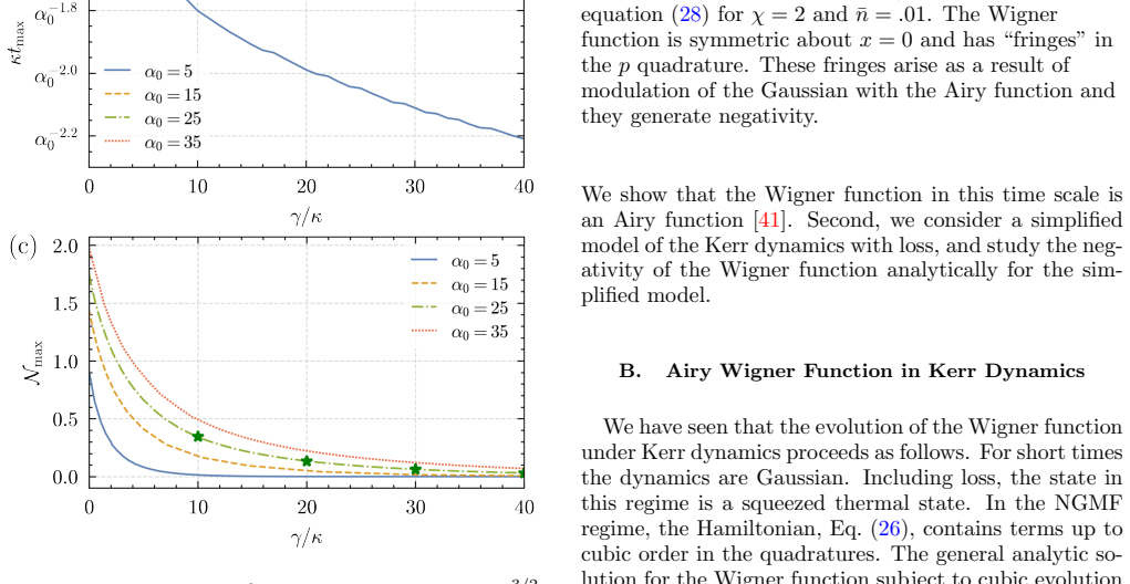
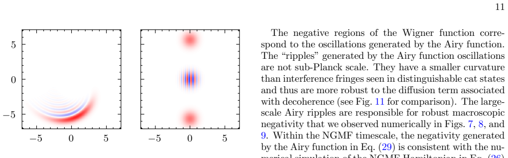
The paper's central claim is that in the non-Gaussian mean-field regime—times around κt ~ 1/α0^(3/2), after squeezing but before sub-Planck kitten structure forms—the open Kerr dynamics produces a Wigner function with robust negative fringes. These fringes are Airy-function oscillations, not fine interference fringes, so photon-loss diffusion washes them out slowly. The paper derives an analytic bound for a squeezing-plus-cubic model, N = exp[-(1+2\bar n)^3/(12χ̃^2)] Ξ(\bar n,χ̃), and shows the damping factor stays order one when γ/κ grows no faster than α0; the effective cubic nonlinearity χ̃ grows like α0^(3/2) while the effective thermal photon number \bar n vanishes in the Gaussian stage
What carries the argument
The load-bearing object is the non-Gaussian mean-field Hamiltonian, Eq. (26): κα0^2 X̂^2 + (κα0/√2)(X̂^3 + P̂X̂P̂ - 2X̂), the first cubic correction to the Gaussian shearing dynamics. Its unitary part generates a Wigner function that is a Gaussian envelope times an Airy function—the 'Airy Wigner function'—whose broad ripples are the source of negativity. To extract scaling analytically, the paper replaces the full dynamics with a two-stage circuit: lossy Gaussian squeezing for κt = c_g/α0^(3/2), then a cubic phase gate with effective strength χ̃ = 3c_a/√2 exp(-c_a γ/(2κ α0)) e^(3r), where e^r ∝ √α0. The formula N = exp[-(1+2\bar n)^3/(12χ̃^2)] Ξ(\bar n,χ̃), with Ξ an 'undamped negativity' th
Load-bearing premise
The load-bearing premise is that the 'undamped negativity' factor Ξ(\bar n,χ̃) left after factoring out the exponential damping stays of order one as α0→∞, and that the simplified squeezing-plus-cubic circuit upper-bounds the full non-Gaussian mean-field dynamics; the paper proves only a polynomial upper bound on Ξ and simulates amplitudes only up to α0=35.
What would settle it
Compute or bound Ξ(\bar n,χ̃) from below as α0→∞, or simulate the non-Gaussian mean-field master equation at amplitudes well beyond α0=35 with fixed γ/κ and see whether the peak Wigner negativity at κt≈α0^(-3/2) decays. If it decays, the central claim fails. Experimentally, measure the Wigner function of a lossy Kerr oscillator at that time for α0 from 20 to 100 and check whether integrated negativity grows with α0.
If this is right
- If the claim holds, the quantum-to-classical transition of the Kerr oscillator is not uniform: the intermediate non-Gaussian regime remains nonclassical even as both earlier and later regimes become classical.
- A coherent state sent through a lossy Kerr medium would deterministically yield a cubic-phase-like state with order-one Wigner negativity at times κt ~ α0^(-3/2), without post-selection.
- Classical simulation by sampling phase-space quasiprobabilities becomes inefficient in this regime, because the negativity of the Wigner function prevents a positive-definite sampling distribution from matching the true state.
- The time window of nonclassicality narrows and shifts toward t=0 as α0 grows; in the infinite-amplitude limit the paper expects a delta-spike in negativity at t=0 for fixed γ.
- Recovering classical flow in the macroscopic limit requires engineering loss that scales faster than amplitude, γ/κ ≳ k α0^(1+ε), rather than merely making the loss rate small.
Where Pith is reading between the lines
- Editorial inference: the Airy-fringe mechanism should be generic; any single-mode nonlinear oscillator whose first anharmonic correction is cubic—self-phase modulation, trapped particles, optomechanics—should show the same three regimes and similar robust negativity, though the paper only asserts this qualitatively.
- Editorial inference: the same scaling suggests a quantitative experimental test: hold γ/κ fixed, prepare coherent states with increasing amplitude, and reconstruct the Wigner function at κt ≈ α0^(-3/2); the integrated negativity should increase with α0, a signature that would not be expected from standard decoherence lore.
- Editorial inference: if the negativity survives at fixed loss, then for sampling-based classical simulation the hard-to-sample region is not the kitten regime (where loss is fatal) but the earlier time window; resource estimates for quantum advantage in Kerr-based continuous-variable devices should focus there.
Editorial analysis
A structured set of objections, weighed in public.
Referee Report
Summary. The paper studies the single-mode Kerr oscillator with photon loss and partitions the dynamics into three regimes: short-time Gaussian, intermediate non-Gaussian mean-field (NGMF), and long-time distinguishable-kitten/sub-Planck. The central claim is that in the NGMF regime, Wigner negativity is robust to loss and persists, and even grows, as the initial coherent-state amplitude α0 → ∞ for fixed loss rate γ; classicality is recovered only when γ/κ ≳ α0^{1+ε}. The authors support this with an exact Fock-basis Wigner solution, a cubic/NGMF Hamiltonian, an Airy-function approximation to the Wigner function, a simplified squeezing-plus-cubic circuit model, and finite-difference numerics up to α0 ≈ 35.
Significance. If established, the result is significant: it provides a concrete counterexample to the usual expectation that weak decoherence always suppresses nonclassical phase-space features in the macroscopic limit, and it has implications for continuous-variable quantum information and classical simulability. The paper has real strengths: the central scaling law is derived from the Hamiltonian rather than fitted to numerics; the Airy approximation is benchmarked against exact or NGMF numerics with order-10% error (Fig. 14); and the analysis of kitten-state fragility is careful. However, the macroscopic-persistence claim is currently an extrapolation: the analytic argument proves only an upper bound on the undamped negativity and therefore does not yet establish that the negativity survives as α0 → ∞.
major comments (2)
- [Sec. V.C, Eq. (35); Appendix F, Eqs. (F25)–(F30)] The central asymptotic claim is not established. Eq. (35) has the product form N = exp[-(1+2nbar)^3/(12χ~^2)] Ξ(nbar,χ~). For γ/κ = k α0^p with p ≤ 1, the exponential prefactor tends to 1, but the total negativity is controlled by the undamped-negativity factor Ξ. Appendix F proves only an upper bound on Ξ, polynomial in χ~. Since χ~ grows with α0 through Eq. (33), an upper bound is fully compatible with Ξ → 0, e.g. Ξ ~ χ~^{-δ} with δ > 0, which would make N vanish despite the prefactor being O(1). The numerics in Figs. 7–9 and Fig. 14 reach α0 ≤ 35 (and the exact benchmark is at α0 = 10), so they cannot distinguish a nonzero limit from slow polynomial decay. A lower bound on Ξ, or a direct asymptotic evaluation of the Airy-negativity integral, is needed before the persistence claim can be made.
- [Sec. V.C, paragraph after Eq. (30)] The simplified circuit model is introduced as being 'a good upper bound of the negativity for NGMF dynamics', but this statement is not proved. This matters for two reasons. First, the scaling conclusions (36)–(37) are derived from the simplified model, not from the NGMF Hamiltonian in Eq. (26). Second, an upper bound on the actual negativity cannot certify persistence: if the simplified model overestimates the negativity, the actual negativity could be much smaller and could vanish even when the model's negativity is O(1). To support the central claim, the authors need either a matching lower bound on the actual NGMF negativity, or an analytic derivation of the asymptotic behavior directly from the Airy Wigner function in Eq. (29).
minor comments (5)
- [Sec. V, opening paragraph] 'For times κt ≳ α0^{1.5}' should presumably be κt ≳ 1/α0^{3/2} (or α0^{-3/2}); as written the inequality has incompatible dimensions for a dimensionless time.
- [Global] Typos: 'Enhrenfest' in the Introduction should be 'Ehrenfest'; 'equaiton' in Appendix B should be 'equation'.
- [Fig. 8 caption] The caption says 'The nonlinearity is plotted as a function of time', but the figure shows Wigner negativity; please rephrase.
- [Sec. V.B] The text says the Airy result is 'consistent with ... the exact Wigner function in Eq. (29)', but Eq. (29) is the approximate Airy Wigner function, not an exact solution. Please clarify which expression is meant to be exact.
- [Availability] No data/code availability statement is included for the numerical simulations. Given the central role of the numerics for α0 up to 35, a statement about reproducibility would strengthen the paper.
Circularity Check
No circular derivation: the central scaling law is analytic and parameter-free; the missing lower bound on the undamped negativity is a rigor gap, not circularity.
full rationale
The central claim—negativity persists unless γ/κ scales faster than α0—is not obtained by fitting or by renaming a fitted quantity. Equation (35) is derived analytically in Appendix F for an explicit circuit model (squeezing followed by cubic nonlinearity), with the effective nonlinearity and thermal photon number taken from the independently derived covariance matrix of Sec. III. The asymptotic threshold follows from evaluating the exponential prefactor for γ/κ = k α0^p; no parameter is adjusted to the numerics to produce the persistence law. The only author self-citation ([28], Propp et al.) is used for the known moment-recurrence signature of kitten states, and that result is also attributed to independent reference [15]; it is not load-bearing for the robust-negativity scaling. The skeptical concern about Sec. V.C / Appendix F is real but is a proof gap, not circularity: the paper bounds the undamped negativity Ξ only from above (polynomially in χ̃) and never proves the needed lower bound, and the statement that the simplified squeezing-plus-cubic model 'will be a good upper bound of the negativity for NGMF dynamics' is asserted without proof. An upper bound cannot certify persistence, and the numerics extend only to α0 = 35, so the macroscopic limit is not fully established. These are correctness/rigor limitations: they weaken the proof, but they do not make Eq. (35) equivalent to an input, a fitted parameter, or a self-citational assumption. No specific circular reduction can be exhibited, so the circularity score is 0.
Axiom & Free-Parameter Ledger
free parameters (5)
- c_g =
unspecified (≪1)
- c_a =
unspecified (≪1)
- k =
positive constant (unspecified)
- α_c =
3/√2 ≈ 2.12
- ε =
0 < ε ≤ 1/2
axioms (6)
- domain assumption The open-system dynamics is governed by the Lindblad master equation (4) with amplitude damping rate γ.
- ad hoc to paper The mean-field non-Gaussian Hamiltonian H_NGMF = κ α0^2 X^2 + (κ α0/√2)(X^3 + P X P − 2X) captures the first non-Gaussian corrections.
- ad hoc to paper The simplified circuit model (lossy Gaussian evolution followed by a pure cubic phase gate along the anti-squeezed quadrature) is a good upper bound for the negativity of the NGMF dynamics.
- domain assumption The Airy Wigner function (Eq. 29) derived under the Bessel approximation (E7) and the condition t ≪ 1/α0 remains valid in the NGMF regime for all α0.
- standard math Hudson's theorem: non-Gaussian pure states have negative Wigner function.
- standard math The identity (E11) for the Airy integral and the asymptotic properties of Ai(x).
read the original abstract
We quantify the quantum-to-classical transition of the single-mode Kerr nonlinear dynamics in the presence of loss. We establish three time scales that govern the dynamics, each with distinct characteristics. For times short compared to the Ehrenfest time, the evolution is classical, characterized by Gaussian dynamics. For sufficiently long times, as we increase the initial photon number, unitary Kerr evolution would generate macroscopic superpositions of coherent states (so-called kitten states), but this is severely restricted in the presence of small photon loss so that expectation values of observables coincide with their classical values. The intermediate time scale, however, shows resilient quantum behavior in the macroscopic limit. We show that in the mean-field non-Gaussian regime, the Kerr Hamiltonian (with small photon loss) generates a significant amount of Wigner-negativity, and classical flow is recovered only if the loss rate grows with system size. Our results broaden the usual understanding of quantum-to-classical transitions and demonstrate the potential for creating robust nonclassical resources for continuous-variable quantum information processing in the presence of loss.
Figures




Reference graph
Works this paper leans on
-
[1]
W. H. Zurek, Reviews of modern physics75, 715 (2003)
2003
-
[2]
For a givenα 0 ≥2, the arc-length around the circle is 2 √ 2πα0 (recall that x0 = √ 2α0), therefore Nmax ≡ ⌊2 √ 2πα0/αc⌋=⌊2πα 0/3⌋.(20) As an example,α 0 = 6 leads toN max = 12
We choose 2αc ≈6∆α≳3 to leave sufficient space for inter- ference terms, as seen in Figure 2. For a givenα 0 ≥2, the arc-length around the circle is 2 √ 2πα0 (recall that x0 = √ 2α0), therefore Nmax ≡ ⌊2 √ 2πα0/αc⌋=⌊2πα 0/3⌋.(20) As an example,α 0 = 6 leads toN max = 12. This is evidenced in Fig. 3, where the 12-kitten state shows the limit in which the i...
-
[3]
boomerang
Asγ/κ increases, the fraction of the kitten state that survives (ns) decreases exponentially inα 0, signifying the fragility of the kitten states to loss. andγ, ns = exp −N 2 maxκ3α2 0 1−e −2πγ Nmax κ −π(γ 3 +N 2 maxκ2γ) κ(γ2 +N 2maxκ2) . (22) We plot this in Fig. 5 as a function ofγ/κfor four dif- ferentα 0 values. It is clear that as we incr...
-
[4]
4a, we plot|⟨α n⟩ − ⟨ˆan⟩|/αn 0 forn= 5 with γ/κ= 10 −4
In Fig. 4a, we plot|⟨α n⟩ − ⟨ˆan⟩|/αn 0 forn= 5 with γ/κ= 10 −4. It is clear that even for such a small loss rate and for largeα 0 (e.g.α 0 = 100), the classical and quantum moments of the open systems barely differ. We observe a similar behavior in quadratures⟨ ˆX 2⟩and⟨ ˆX 5⟩ in Fig. 4b. These quadratures were calculated using ap- propriately ordered ex...
-
[5]
W. H. Zurek and J. P. Paz, Physical Review Letters72, 2508 (1994)
1994
-
[6]
W. H. Zurek, Physica Scripta1998, 186 (1998)
1998
-
[7]
drift term
However, the full-master equation is difficult to simu- late for largeα 0. Moreover, it is numerically challenging to extract negativity from the general solutions. To mit- igate this, we simulate the system dynamics using the NGMF approximation to the Hamiltonian, ˆHNGMF, and the Lindbladian for loss. In the Wigner-Weyl representa- tion, the equation of ...
-
[8]
J. E. Moyal, inMathematical Proceedings of the Cam- bridge Philosophical Society, Vol. 45 (Cambridge Univer- sity Press, 1949) pp. 99–124
1949
-
[9]
(29) is consistent with the nu- merical simulation of the NGMF Hamiltonian in Eq
Within the NGMF timescale, the negativity generated by the Airy function in Eq. (29) is consistent with the nu- merical simulation of the NGMF Hamiltonian in Eq. (26) and with the exact Wigner function in Eq. (29), as seen in Fig. 14 in Appendix E. C. Scaling of Robust Macroscopic Negativity The Airy Wigner function given in Eq. (29) sheds light on the ex...
-
[10]
W. H. Zurek, Physics today44, 36 (1991)
1991
-
[11]
J. P. Paz, S. Habib, and W. H. Zurek, Physical Review D47, 488 (1993)
1993
-
[12]
B. D. Greenbaum, S. Habib, K. Shizume, and B. Sun- daram, Chaos: An Interdisciplinary Journal of Nonlinear Science15(2005)
2005
-
[13]
Habib, K
S. Habib, K. Shizume, and W. H. Zurek, Physical review letters80, 4361 (1998)
1998
-
[14]
I. Katz, A. Retzker, R. Straub, and R. Lifshitz, Physical review letters99, 040404 (2007)
2007
-
[15]
J. Galkowski and M. Zworski, arXiv preprint arXiv:2403.09345 (2024)
Pith/arXiv arXiv 2024
-
[16]
Hern´ andez, D
F. Hern´ andez, D. Ranard, and C. J. Riedel, Communi- cations in Mathematical Physics406, 4 (2025)
2025
-
[17]
F. Hern´ andez, D. Ranard, and C. J. Riedel, arXiv preprint arXiv:2306.13717 (2023)
Pith/arXiv arXiv 2023
-
[18]
Preskill, Quantum2, 79 (2018)
J. Preskill, Quantum2, 79 (2018)
2018
-
[19]
Tanas, Theory of Nonclassical States of Light , 277 (2003)
R. Tanas, Theory of Nonclassical States of Light , 277 (2003)
2003
-
[20]
K. Tara, G. Agarwal, and S. Chaturvedi, Physical Re- view A47, 5024 (1993)
1993
-
[21]
Miranowicz, R
A. Miranowicz, R. Tanas, and S. Kielich, Quantum Op- tics: Journal of the European Optical Society Part B2, 253 (1990)
1990
-
[22]
Stobi´ nska, G
M. Stobi´ nska, G. J. Milburn, and K. W´ odkiewicz, Open Systems & Information Dynamics14, 81 (2007)
2007
-
[23]
L. Ar´ evalo-Aguilar, R. Ju´ arez-Amaro, J. Vargas- Martinez, O. Aguilar-Loreto, and H. Moya-Cessa, arXiv preprint arXiv:0806.4146 (2008)
Pith/arXiv arXiv 2008
-
[24]
Chaturvedi and V
S. Chaturvedi and V. Srinivasan, Physical Review A43, 4054 (1991)
1991
-
[25]
Peinova and A
V. Peinova and A. Luk, Physical Review A41, 414 (1990)
1990
-
[26]
G. J. Milburn and C. A. Holmes, Physical review letters 56, 2237 (1986)
1986
-
[27]
Daniel and G
D. Daniel and G. Milburn, Physical Review A39, 4628 (1989)
1989
-
[28]
K¨ artner and A
F. K¨ artner and A. Schenzle, Physical Review A48, 1009 (1993)
1993
-
[29]
McDonald and A
A. McDonald and A. A. Clerk, Physical Review Letters 128, 033602 (2022)
2022
-
[30]
McDonald and A
A. McDonald and A. A. Clerk, Physical Review Research 5, 033107 (2023)
2023
-
[31]
Villegas-Mart ´ ınez, F
B. Villegas-Mart ´ ınez, F. Soto-Eguibar, and H. Moya- Cessa, Advances in Mathematical Physics2016, 9265039 15 (2016)
2016
-
[32]
Stobi´ nska, G
M. Stobi´ nska, G. Milburn, and K. W´ odkiewicz, Physical Review A—Atomic, Molecular, and Optical Physics78, 013810 (2008)
2008
-
[33]
T. B. Propp, S. Ray, J. B. DeBrota, T. Albash, and I. H. Deutsch, Physical Review A108, 062219 (2023)
2023
-
[34]
Agasti, Journal of Physics Communications3, 105004 (2019)
S. Agasti, Journal of Physics Communications3, 105004 (2019)
2019
-
[35]
Verstraelen and M
W. Verstraelen and M. Wouters, Applied Sciences8, 1427 (2018)
2018
-
[36]
Van Enk, Physical Review A—Atomic, Molecular, and Optical Physics72, 022308 (2005)
S. Van Enk, Physical Review A—Atomic, Molecular, and Optical Physics72, 022308 (2005)
2005
-
[37]
R. G. Corti˜ nas, New Journal of Physics26, 023022 (2024)
2024
-
[38]
G. J. Milburn, Physical Review A33, 674 (1986)
1986
-
[39]
Although the real moments go to zero classically, Kerr dynamics preserve absolute variance⟨∆|α| 2⟩, which de- pend on⟨α ∗α⟩
-
[40]
Kartner, L
F. Kartner, L. Joneckis, and H. Haus, Quantum Optics: Journal of the European Optical Society Part B4, 379 (1992)
1992
-
[41]
Osborn and K.-P
T. Osborn and K.-P. Marzlin, Journal of Physics A: Mathematical and Theoretical42, 415302 (2009)
2009
-
[42]
Polkovnikov, Annals of Physics325, 1790 (2010)
A. Polkovnikov, Annals of Physics325, 1790 (2010)
2010
-
[43]
Mari and J
A. Mari and J. Eisert, Physical review letters109, 230503 (2012)
2012
-
[44]
C. A. Rosiek,Enhancing the Formation of Wigner Neg- ativity in a Kerr Oscillator Via Quadrature Squeezing (Niels Bohr Institute, Copenhagen University, 2019)
2019
-
[45]
R. L. Hudson, Reports on Mathematical Physics6, 249 (1974)
1974
-
[46]
Vall´ ee and M
O. Vall´ ee and M. Soares,Airy functions and applications to physics(World Scientific, 2010)
2010
-
[47]
D. W. Moore and R. Filip, arXiv preprint arXiv:2504.04851 (2025)
arXiv 2025
-
[48]
D. Gottesman, A. Kitaev, and J. Preskill, arXiv preprint quant-ph/0008040 (2000)
Pith/arXiv arXiv 2000
-
[49]
Ghose and B
S. Ghose and B. C. Sanders, Journal of Modern Optics 54, 855 (2007)
2007
-
[50]
Albarelli, M
F. Albarelli, M. G. Genoni, M. G. Paris, and A. Ferraro, Physical Review A98, 052350 (2018)
2018
-
[51]
Yanagimoto, T
R. Yanagimoto, T. Onodera, E. Ng, L. G. Wright, P. L. McMahon, and H. Mabuchi, Physical Review Letters 124, 240503 (2020)
2020
-
[52]
Br¨ auer and P
ˇS. Br¨ auer and P. Marek, Optics Express29, 22648 (2021)
2021
-
[53]
V. Kala, R. Filip, and P. Marek, Optics Express30, 31456 (2022)
2022
-
[54]
Riera-Campeny, M
A. Riera-Campeny, M. Roda-Llordes, P. T. Grochowski, and O. Romero-Isart, Quantum8, 1393 (2024)
2024
-
[55]
Neumeier, M
L. Neumeier, M. A. Ciampini, O. Romero-Isart, M. As- pelmeyer, and N. Kiesel, Proceedings of the National Academy of Sciences121, e2306953121 (2024)
2024
-
[56]
Pashayan, J
H. Pashayan, J. J. Wallman, and S. D. Bartlett, Physical review letters115, 070501 (2015)
2015
-
[57]
Temme, S
K. Temme, S. Bravyi, and J. M. Gambetta, Physical review letters119, 180509 (2017)
2017
-
[58]
Zheng, O
Y. Zheng, O. Hahn, P. Stadler, P. Holmvall, F. Qui- jandr ´ ıa, A. Ferraro, and G. Ferrini, PRX Quantum2, 010327 (2021)
2021
-
[59]
O. Hahn, P. Holmvall, P. Stadler, G. Ferrini, and A. Fer- raro, Physical Review A105, 062446 (2022)
2022
-
[60]
J. Guo, S. Liu, B. Jing, Q. He, and M. Gessner, arXiv preprint arXiv:2512.03769 (2025), arXiv:2512.03769 [quant-ph]
arXiv 2025
-
[61]
J. E. Bourassa, R. N. Alexander, M. Vasmer, A. Patil, I. Tzitrin, T. Matsuura, D. Su, B. Q. Baragiola, S. Guha, G. Dauphinais,et al., Quantum5, 392 (2021)
2021
-
[62]
Takase, F
K. Takase, F. Hanamura, H. Nagayoshi, J. E. Bourassa, R. N. Alexander, A. Kawasaki, W. Asavanant, M. Endo, and A. Furusawa, Phys. Rev. A110, 012436 (2024)
2024
-
[63]
H. M. Vasconcelos, L. Sanz, and S. Glancy, Opt. Lett. 35, 3261 (2010)
2010
-
[64]
Konno, W
S. Konno, W. Asavanant, F. Hanamura, H. Nagayoshi, K. Fukui, A. Sakaguchi, R. Ide, F. China, M. Yabuno, S. Miki,et al., Science383, 289 (2024)
2024
-
[65]
P. L. Voss, K. G. K¨ opr¨ ul¨ u, and P. Kumar, J. Opt. Soc. Am. B23, 598 (2006)
2006
-
[66]
Z. Zhang, X.-Q. Dinh, and P. L. Voss, Journal of Modern Optics58, 988 (2011), https://doi.org/10.1080/09500340.2011.589915
arXiv 2011
-
[67]
Vitali, P
D. Vitali, P. Tombesi, and P. Grangier, Applied Physics B64, 249 (1997)
1997
-
[68]
NIST Digital Library of Mathematical Func- tions,
DLMF, “NIST Digital Library of Mathematical Func- tions,”https://dlmf.nist.gov/, Release 1.2.4 of 2025- 03-15, f. W. J. Olver, A. B. Olde Daalhuis, D. W. Lozier, B. I. Schneider, R. F. Boisvert, C. W. Clark, B. R. Miller, B. V. Saunders, H. S. Cohl, and M. A. McClain, eds
2025
-
[69]
Matlab version: 23.2.0.2428915 (r2023b),
T. M. Inc., “Matlab version: 23.2.0.2428915 (r2023b),” (2023)
2023
-
[70]
I. S. Gradshte ˘ ın and D. Zwillinger,Table of integrals, se- ries, and products, eighth edition ed. (Elsevier, Academic Press is an imprint of Elsevier). Appendix A: Squeezing with loss In the Heisenberg-Langevin picture the equation of motion for the annihilation operator according to Kerr Hamil- tonian is dˆa dt =− γ 2 ˆa−iκˆa†ˆaˆa+ˆF(A1) where the Lan...
-
[71]
diagonal terms
Wigner F unction of Kitten States Given a state of the form|ψ⟩= PN k=1 ck |αk⟩(where|α k⟩are coherent states), the Wigner function of|ψ⟩is given by: W|ψ⟩(β, β∗) = 2 π N,NX k,l=0 ckc∗ l e 1 2 (4(−β+αk)β∗−|αk|2−(−4β+2αk+αl)α∗ l ). (C1) From the definition ofN-kitten states in Eq. (19), the Wigner function ofN-kitten states is given by: W(β) = N−1X j,k=0 cjc...
-
[72]
Since these circles depend on the difference ofkandj, these circles exist on radiir ℓ =α 0 p 2 + 2 cos (2πl/N)/2 = α0 cos (πℓ/N), whereℓ∈ {0,
Strong Distinguishability Letz j,k ≡(α j +α k)/2, the phasorsz j,k all lie on concentric circles of radii|z j,k|2 =α 2 0(2 + 2 cos(2π(k−j)/N))/4. Since these circles depend on the difference ofkandj, these circles exist on radiir ℓ =α 0 p 2 + 2 cos (2πl/N)/2 = α0 cos (πℓ/N), whereℓ∈ {0, . . . ,(N−1)/2}. The distances between neighboring concentric circles...
-
[73]
First, we derive an upper-bound and follow with a derivation of a lower-bound
Negativity of Strongly Distinguishable Kitten State Now we use the definition of strong distinguishability to bound the negativity of the kitten state. First, we derive an upper-bound and follow with a derivation of a lower-bound. a. Upper-Bound: Recall the definition of negativity, N= Z (|W(β)| −W(β))d2β= Z X jk Wjk (β) d2β−1.(C11) Applying the triangle ...
-
[74]
As elsewhere, we takeα 0 real, soϕ 0 = 0. The Wigner function for this state is given by substituting the Weyl symbol for|n⟩ ⟨m|, equation (9) reproduced here in polar coordinates Wn,m(r, ϕ) =2 π (−1)n r n! m! (2r)m−ne−2r2 e−iϕ(m−n)Lm−n n (4r2),(E2) to obtain W(r, ϕ, t) =2 π e−2r2−r2 0 ∞X n,m=0 (−1)n m! rn+m 0 (2r)m−ne−iϕ(m−n)e −it 2 (m(m−1)−n(n−1)) ×e − ...
discussion (0)
Sign in with ORCID, Apple, or X to comment. Anyone can read and Pith papers without signing in.