Quantum cosmological perturbations in bouncing models with mimetic dark matter

D\^eivid R. da Silva; Idaiane L. Machado; Nelson Pinto-Neto

REVIEW 3 major objections 5 minor 44 references

Quantum cosmological perturbations in bouncing models with mimetic dark matter

T0 review · 3 major / 5 minor · reviewed 2026-08-07 · deepseek-v4-flash

Challenge this review Re-run · record.json Download PDF Read on arXiv ↗

Pith's one-line read Mimetic dark matter bouncing models can generate the observed primordial perturbation spectrum without inflation and without quantum gravity.

desk verdict Solid background work on mimetic bounces, but the scale-invariance claim rests on a k-matching step that looks wrong, and the numerics inherit a flat spectrum from a k-independent initial condition. read the letter →

arxiv 2506.06901 v2 pith:AICCT4JS submitted 2025-06-07 astro-ph.CO gr-qchep-th

Idaiane L. Machado , Dêivid R. da Silva , Nelson Pinto-Neto This is my paper

classification astro-ph.COgr-qchep-th PACS 98.80.Bp98.80.Cq

keywords DarkMatterBouncingCosmologyPowerSpectrumNon-standardmimeticgravitycosmologicalperturbationsquantumvacuumfluctuationsspectralindex

verification ladder T0 review T1 audit T2 compute T3 formal

The pith

A machine-rendered reading of the paper's core claim, the machinery that carries it, and where it could break.

The reading

This paper argues that bouncing cosmologies built from mimetic dark matter can generate the primordial perturbation spectrum measured in the cosmic microwave background, without inflation and without quantum gravity. It computes the power spectrum of scalar perturbations starting from quantum vacuum fluctuations in the contracting phase and finds a scale-invariant spectrum. The amplitude fixes the bounce length scale to the interval $10^5 l_p < t_0 < 10^9 l_p$, values large enough to stay away from Planck-scale physics and small enough to avoid nucleosynthesis. A slight deformation of the mimetic potential yields the observed red tilt, $n_s \approx 0.965$, without introducing negative pressure or an unstable sound speed. If correct, the mimetic bounce becomes a viable non-inflationary source of structure.

What carries the argument

The load-bearing object is the scalar power spectrum $\delta^2_\psi(k)=k^3/(2\pi^2)|\psi_k|^2$, with the Newtonian potential $\psi$ linked to the mimetic field perturbation by $\psi=\delta\dot\phi$ through the mimetic constraint. The mode equation for the canonical variable $v\propto k\,\delta\phi_k$ is $v''+[c_s^2 k^2+a''/a-2(a'/a)^2]v=0$, where primes are conformal-time derivatives. Adiabatic vacuum initial conditions in the asymptotic past select the mode function, and matching to the long-wavelength solution $v=(1/a)(A_1+A_2\int a^2\,d\eta)$ yields $A_1\propto k^{-5/2}$; since $\delta^2_\psi\propto k^3(kA_1)^2$, the $k$-dependence cancels and the spectrum is scale invariant. The amplitude then depends on $t_0$ through $\delta^2_\psi=(c_s/(2\gamma))(l_p^2/t_0^2)\delta^2_{\psi,\mathrm{num}}$, converting the observed amplitude into a constraint on the bounce scale.

What would settle it

Measure the scalar spectral index and amplitude at percent level and solve the amplitude relation $\delta^2_\psi=(c_s/(2\gamma))(l_p^2/t_0^2)\delta^2_{\psi,\mathrm{num}}$ for $t_0$ from the observed $\delta^2_\psi$; the model is falsified if $t_0$ falls outside $10^5 l_p < t_0 < 10^9 l_p$. A detection of a running spectral index or of non-Gaussianity incompatible with a single scalar field in the adiabatic vacuum would also violate the setup.

Watch

Extended reading notes

Core claim

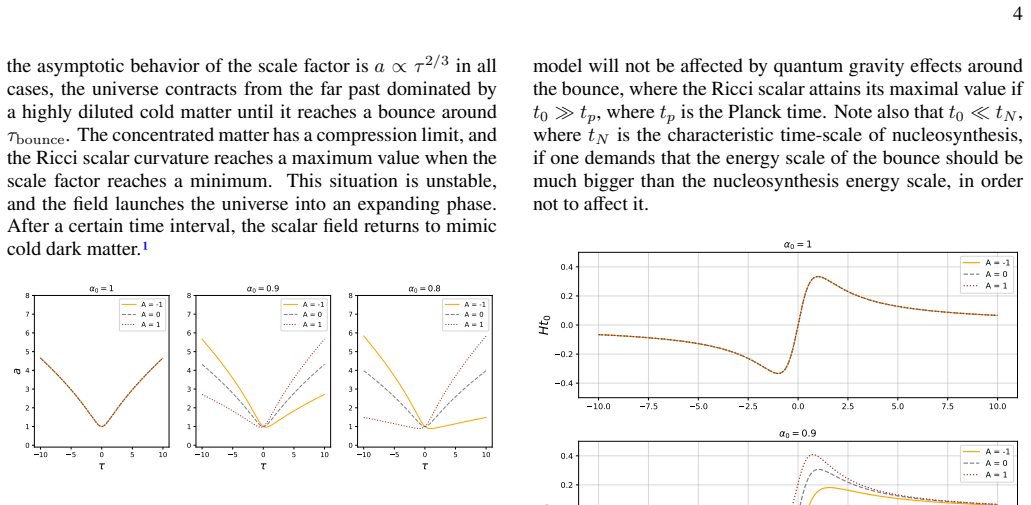
Read at face value, the paper shows that the observed scalar power spectrum can be produced by a nonsingular, purely classical bounce in mimetic gravity. Starting from the bounce solutions $a(\tau)=a_b(1+\tau^2)^{1/3}[\cos(\beta\arctan\tau)+A\sin(\beta\arctan\tau)]^{2/3}$, it quantizes the canonical perturbation variable $v\propto k\,\delta\phi_k$, imposes the adiabatic vacuum on sub-Hubble scales in the asymptotic past, and matches the vacuum mode onto the long-wavelength solution across the bounce. The matching gives $A_1\propto k^{-5/2}$, so the spectrum $\delta^2_\psi\propto k^3(kA_1)^2$ is scale invariant for the parameter range considered. The amplitude is $\delta^2_\psi = (c_s/(2\gamma))(l_p^2/t_0^2)\delta^2_{\psi,\mathrm{num}}$; with the observationally allowed sound speed $c_s=\sqrt{\gamma}=10^{-5}$ and the measured $\delta^2_\psi\approx 10^{-9}$, the bounce scale must satisfy $10^5 l_p < t_0 < 10^9 l_p$. With a modified potential the scale factor becomes $a(\tau)=a_b(1+\tau^2)^{1/[3(1+w)]}$, giving the spectral index $n_s=1+12w/(1+3w)$, whose small negative $w$ reproduces the observed red tilt.

Load-bearing premise

The calculation assumes that deep in the contracting phase the perturbations begin as adiabatic quantum vacuum fluctuations on sub-Hubble scales; if the initial state differed, the predicted amplitude and spectral index would change.

Editorial extensions

If this is right

The observed scalar spectrum can be matched with a purely classical bounce, so no background quantum effect is required when the bounce scale lies in $10^5 l_p < t_0 < 10^9 l_p$.
The measured amplitude effectively fixes the bounce scale $t_0$, turning it from a free parameter into a testable prediction.
A red tilt $n_s\approx 0.965$ follows from a small negative $w$ in the mimetic potential, without introducing negative pressure or an unstable sound speed.
Scale invariance holds across the single-bounce family parameterized by $0.75\le\alpha_0\le 1$ and $-1\le A\le 1$.
The power spectrum is tied to quantum vacuum fluctuations in the asymptotic past, so the model inherits the standard vacuum choice of bouncing cosmologies.

Reading between the lines

Editorial extensions of the paper, not claims the author makes directly.

The paper does not compute the tensor power spectrum; under the same vacuum initial condition and matching, one would expect a gravitational-wave background whose amplitude also depends on $t_0$, giving an additional observational test.
The matching that fixes $A_1$ could be replaced by a direct numerical integration of the full mode equation through the bounce, providing an independent check on $A_1\propto k^{-5/2}$.
The relation $n_s=1+12w/(1+3w)$ implies that a precision measurement of $n_s$ would determine $w$ directly, linking the bounce potential to CMB data.

Share X Bluesky LinkedIn Reddit HN

Editorial analysis

A structured set of objections, weighed in public.

Desk editor's note, referee report, and a circularity audit.

Desk Editor's Note

read the letter

Short version: the background part is good and the paper is clearly written, but I do not think the central scale-invariance result is established. The matching step in Sec. 4A has a k-dependence problem, and the numerical flatness looks baked into the initial conditions. The reader's conditional verdict is generous.

What is new: the paper takes the known Peter-Pinto-Neto matter-bounce calculation and applies it to the mimetic backgrounds of Chamseddine-Mukhanov-Vikman, including the asymmetric family 0.75 <= alpha0 < 1, and it adds a modified potential to get a red tilt. The background analysis in Eqs. (19)-(28), the classification of bounces, and the plots of H, rho, and R are careful and useful. The alpha0 = 1 case correctly reduces to the PPN result, and the reduction to the canonical variable and adiabatic vacuum is standard.

The soft spot is load-bearing. In the super-Hubble limit, Eq. (44) behaves as eta^-2 with a coefficient proportional to k^-3/2. Matching to Eq. (45) gives A1 proportional to k^-3/2, not the k^-5/2 the text claims. Plugging A1 proportional to k^-3/2 into their own Eq. (52) gives delta^2_psi proportional to k^2, not scale invariant. I do not see where the extra k^-1 comes from. The numerical calculation has the same problem in disguise: the initial condition (56b) is k-independent, and since c_s kbar is 10^-22 to 10^-17 in the plotted range, the k^2 term in (55b) is negligible, so |pi_num|^2 is flat by construction. That is not evidence for scale invariance; it is an artifact of the initial condition.

The red-tilt section is thinner. Eq. (65) is stated without derivation, and choosing omega to hit n_s = 0.965 is a fit. That is acceptable for model-building, but it should be labeled as such. The amplitude constraint t0 in [10^5, 10^9] l_p is broad and has no error bars, so it is not a sharp test.

Citation pattern is fine; the comparison to Ref. [26] is the right one. No invented entities. The paper is honest and readable, and the background section alone may be worth something. But as it stands, the abstract's claim that all physically relevant models produce scale-invariant spectra with observed amplitude is not supported by the calculation shown.

I would not cite this as is. It does deserve a serious referee: if the k-scaling can be fixed, or if I am missing a legitimate matching surface, this becomes a useful paper. Send to review, but expect major revision on Section 4A. If the authors cannot fix the matching, the central result goes away.

Referee Report

3 major / 5 minor

Summary. This paper studies scalar cosmological perturbations in bouncing scenarios based on mimetic dark matter with the potential V(φ) = (2/3)(2-3γ)α/(t0^2+φ^2)^2 (and a modified version). The authors derive the background bounce solutions, quantize the scalar perturbations with an adiabatic vacuum in the far past, match the vacuum mode to the long-wavelength solution, and compute the power spectrum analytically and numerically. They claim a scale-invariant spectrum for the original potential and an amplitude compatible with Planck for bounce time t0 in 10^5 lp < t0 < 10^9 lp; a red-tilted spectrum n_s = 1 + 12w/(1+3w) is claimed for a slightly modified potential. The paper is clearly organized and presents explicit analytic formulas and numerical solutions.

Significance. If established, the result would constitute an interesting non-inflationary mechanism: a single mimetic scalar field would not only mimic dark matter but also produce the observed primordial spectrum, with the bounce at length scales far above the Planck length, avoiding quantum gravity corrections. The paper is careful in specifying the initial-state assumption and in deriving the background solutions, and the numerical mode equations are explicit and standard. However, the analytic derivation contains a normalization error that is load-bearing for the spectral index, and the red-tilt section conflates background and perturbation integration constants. These issues prevent the claims from being accepted in the present form.

major comments (3)

[Sec. 4A, Eqs. (43)-(45), (52)] Eq. (43) gives the adiabatic vacuum mode as v_k ≈ exp(-i∫ν dη)/√(mν) = l_p√(c_s k) e^{-i c_s k η}. Since m=1/l_p^2 and ν=c_s k, the correct factor is √(mν)=√(c_s k)/l_p, so the amplitude should be l_p/√(c_s k), not l_p√(c_s k). With the printed normalization, taking the super-Hubble limit of Eq. (44) gives v_k ≈ -3 l_p/(c_s^{3/2} k^{3/2} η^2); matching to Eq. (45) with a ∝ η^2 yields A1 ∝ k^{-3/2}, and Eq. (52) then gives δ²_ψ ∝ k^2. With the corrected normalization, v_k ≈ -3 l_p/(c_s^{5/2} k^{5/2} η^2) and A1 ∝ k^{-5/2} as stated. The manuscript is internally inconsistent: Eq. (43) and the subsequent matching cannot both be correct. This must be repaired, and the numerical initial conditions (56), which appear to be consistent with the corrected normalization, should be re-derived explicitly from Eq. (44).
[Sec. 4C, around Eqs. (63)-(65)] After Eq. (63), the text says that the adiabatic vacuum condition selects the mode function (43), 'which corresponds to setting the integration constant C2(k)=0', and that 'using this condition' the scale factor (64) is recovered. The constants C1, C2 in Eq. (63) are integration constants for the background equation (62), not the perturbation-mode coefficients of Eq. (41). The quantum vacuum fixes the perturbation initial state; it does not select a background branch. The choice C2=0 in Eq. (63) is an extra assumption about which bounce solution is realized, and the paper needs to state and justify it. In addition, the spectral index formula (65) is asserted without a derivation or a precise reference, and the relation between w in (61) and an effective equation of state should be explained.
[Sec. 4C, amplitude claim] The sentence 'as |w|≪1, the modification will not modify the amplitudes' is not supported by any calculation in the manuscript. The amplitude analysis in Sec. 4B was performed for the original potential (19) and for specific values of α0 and A (Figs. 5-6). The modified potential (61) changes the background scale factor to (64) for every w≠0, and hence changes the mode equation and the normalization of the power spectrum. An O(w) change in the amplitude is relevant because the quoted interval 10^5 l_p < t0 < 10^9 l_p is derived by matching the numerical amplitude to the Planck value. The authors should either compute the amplitude for the modified potential or show analytically that the w-dependence cancels.

minor comments (5)

[Eq. (35)] The notation '∂iδϕ′∂jδϕ′δij ⊃ S' is confusing; the kinetic term should be written unambiguously (e.g., (∂_i δϕ')^2).
[Eq. (51)] The notation on the left of Eq. (51), 'Hχ k / a ≈ ˙χk/a', is not defined; this quantity is δφdot, and the equation should be written in terms of δφdot.
[After Eq. (60)] The sentence 'scales from the Hubble radius to [42]' appears incomplete.
[Throughout] The symbols w and ω are both used for the new parameter; please use one consistently.
[Figs. 5-6] Figures 5 and 6 do not report numerical tolerances or convergence checks; a brief statement on the ODE solver settings would be useful.

Circularity Check

0 steps flagged · score 1.0 of 10

No significant circularity: the scale-invariant spectrum follows from the adiabatic-vacuum initial conditions and the known matter-bounce mechanism, while the red tilt and the t0 interval are parameter constraints rather than predictions; self-citations support standard techniques but the core derivation is self-contained.

full rationale

The paper's central chain is: (i) solve the mimetic background bounce (Eq. 21), (ii) write the perturbation equation (Eq. 39) and impose the adiabatic vacuum in the asymptotic past via Eq. (43), (iii) match the vacuum mode to the long-wavelength solution (45) to obtain A1 ∝ k^{-5/2} and hence a flat spectrum through Eq. (52), and (iv) integrate numerically the Hamilton equations (55) with initial conditions (56) that are stated to come from Eq. (44). The numerical flatness indeed follows because π_num,in is k-independent and the (cs kbar)^2 term is negligible, but this k-independence is not imposed to fit the final spectrum; it is a consequence of the vacuum mode (44) when expressed in the dimensionless variables (54). That is a physical assumption, not a fitted input called a prediction. The red-tilted result is obtained by the sentence 'Setting w < 0 with the appropriate value, we obtain the observed red tilt' (Sec. 4C), so the parameter ω is tuned to match the measured n_s; the paper carefully says 'obtain' rather than 'predict', making this a parameter constraint rather than a circular prediction. Likewise, the amplitude is used to infer t0 ('we can adjust t0 to give the observed amplitude'), and the abstract reports this as a compatibility interval, not as an independent prediction. The self-citations to Refs. [26], [39], and [40] support standard techniques (adiabatic vacuum, mode dominance in bouncing models) rather than supplying the target result itself; the scale-invariance argument is re-derived in Sec. 4A. Some technical steps, such as the precise k-scaling of A1 and the consistency of the initial conditions with the sub-Hubble vacuum, may warrant scrutiny, but they are correctness risks rather than circular reductions. Overall, the derivation is self-contained and the observable claims are not equivalent to their inputs by construction.

Assumptions & free parameters 5 free parameters · 6 assumptions · 0 invented entities

The central claims rest on the mimetic gravity framework, the choice of vacuum initial conditions, and a set of parameters that are scanned or fitted. The scale-invariance result follows from the matter-dominated contraction asymptotics, while the red tilt is obtained by fitting the potential parameter omega to the observed spectral index. No new physical entities beyond the existing mimetic field and potential are introduced.

free parameters (5)

t0 = 10^5 lp to 10^9 lp (inferred from amplitude)
The bounce length scale is chosen so that the computed amplitude matches the observed delta2_psi approximately 10^-9, giving a range rather than a prediction.
c_s (or gamma) = 10^-5
The sound speed is set to c_s approximately sqrt(gamma) = 10^-5 following Ref. [43]. It directly scales the amplitude via Eq. (58).
omega (w) = approximately -0.003 (to give n_s = 0.965)
The potential modification parameter is chosen so that Eq. (65) yields the observed red-tilted spectral index.
alpha0 = 0.75 to 1 (scanned)
The background potential parameter is restricted to this range to avoid singularities; it affects the asymmetry and amplitude of the power spectrum but not the spectral index.
A = -1 to 1 (scanned)
The asymmetry parameter in the background solution (21) is scanned in this range; it changes the amplitude of delta2_psi,num.

assumptions (6)

domain assumption Mimetic gravity action with constraint g^mu nu partial_mu phi partial_nu phi = 1
The entire paper operates within the mimetic gravity framework introduced in Ref. [3] and developed in Ref. [1]; see Section 2.
domain assumption Homogeneous, isotropic, spatially flat background with phi = t
This is used to derive the Friedmann equation and the background solutions in Sections 2 and 3.
domain assumption The added gamma (box phi)^2 term in the action does not affect the background and yields sound speed c_s^2 = gamma/(2 - 3 gamma)
The term is introduced in Eq. (14) and is claimed to leave the homogeneous background unchanged; the sound speed follows from linearized equations, cited from Refs. [1, 34-36].
domain assumption Adiabatic vacuum initial conditions in the far past
The quantum state is taken as the adiabatic vacuum on sub-Hubble scales in the asymptotic past, following the standard approach in bouncing models; Section 4A.
ad hoc to paper Spectral index formula n_s = 1 + 12 w/(1 + 3 w)
Stated in Eq. (65) without derivation or citation; it is the basis for the red-tilt claim and is not derived from the perturbation equation in the paper.
ad hoc to paper Modified potential (61) is a slight modification for |omega| << 1 and does not change the amplitudes
Introduced in Section 4C to obtain the observed red tilt; the claim that amplitudes are unchanged for small omega is asserted without a detailed calculation.

how reviews work

0 comments

Cite this review

Pith. "Pith review of Quantum cosmological perturbations in bouncing models with mimetic dark matter." pith.science (2026). https://pith.science/paper/AICCT4JS

@misc{pith2026250606901,
  author       = {Pith},
  title        = {Pith review of: Quantum cosmological perturbations in bouncing models with mimetic dark matter},
  year         = {2026},
  howpublished = {\url{https://pith.science/paper/AICCT4JS}},
  note         = {Machine review of arXiv:2506.06901}
}

abstract

We calculate the power spectrum of cosmological perturbations originated from quantum vacuum fluctuations in bouncing scenarios proposed in Ref.~\cite{chamseddine2014cosmology} in the framework of mimetic cosmology. We show that all physically relevant models produce scale invariant spectral indices, and amplitudes compatible with observations provided that the bounce occurs at length scales $t_0$ inside the physically reasonable interval $10^5 l_p < t_0 < 10^9 l_p$. We also show that by slightly modifying the scalar field potential proposed in Ref.~\cite{chamseddine2014cosmology}, we can also obtain the observed red-tilted spectral index, with the same amplitude constraints. Hence, mimetic cosmology provides reasonable bouncing cosmological models without the need of any background quantum effect.

Figures

Figures reproduced from arXiv: 2506.06901 by the authors.

**Figure 1.** Evolution of the factor a with the dimensionless time parameter τ , considering 0.8 ≤ α0 ≤ 1 and −1 ≤ A ≤ 1. All these cases are bouncing scenarios without singularities. Note that for α0 ̸= 1 and A ̸= 0 the models are asymmetric with respect to the bounce, otherwise they are symmetric. In Figures 2 and 3, we plot the Hubble parameter and the energy density of the scalar field, calculated using the Friedmann equati… view at source ↗

**Figure 2.** The Hubble parameter H evolution for models with a unique bounce event around τ ≈ 0. 4. PERTURBATIONS In this section, we will perturb the bouncing models presented in the previous section in order to calculate the power spectrum of scalar cosmological perturbations in such mimetic field scenarios and compare with some observational data. For that, we consider the perturbations in the metric in the Newtonian gauge… view at source ↗

**Figure 3.** The energy density ϵ˜ = H2 evolution for models with a unique bounce event around τ ≈ 0. the following connection between the Newtonian potential and the perturbation of the scalar field: ψ = δϕ.˙ (32) Therefore, to obtain the power spectrum of ψ, which is the one confronted with observations, we only have to calculate the power spectrum of δϕ˙ . Manipulating the first-order terms of the Einstein equations yields th… view at source ↗

Figures from the paper (2 more)

**Figure 5.** Figure 5: , as functions of ¯k, and in [PITH_FULL_IMAGE:figures/full_fig_p007_5.png]

**Figure 6.** Figure 6: The power spectrum δ 2 ψ,num is evaluated for k¯ = {10−17 , 10−16 , 10−15 , 10−14}. The plots show that in the far past and in the far future, the power spectrum is independent of the K value, indicating scale invariance. C. Generalized Potential The primordial scalar …

Discussion (0). Sign in to comment.

Reference graph

Works this paper leans on

44 extracted references · 27 canonical work pages

[26]

Peter and N

P. Peter and N. Pinto-Neto, Phys. Rev. D 78, 063506 (2008), arXiv:0809.2022 [gr-qc]

arXiv 2008
[1]

A. H. Chamseddine, V. Mukhanov, and A. Vikman, Journal of Cosmology and Astroparticle Physics 2014 (06), 017

work page 2014
[2]

G. e. Gu, Dynamical dark energy in light of the desi dr2 baryonic acoustic oscillations measurements (2025), arXiv:2504.06118, arXiv:2504.06118 [astro-ph.CO]

arXiv 2025
[3]

A. H. Chamseddine and V. Mukhanov, Journal of High Energy Physics 2013, 1 (2013)

work page 2013
[4]

Myrzakulov, L

R. Myrzakulov, L. Sebastiani, S. Vagnozzi, and S. Zerbini, Clas- sical and quantum gravity 33, 125005 (2016)

work page 2016
[5]

Vagnozzi, Classical and Quantum Gravity34, 185006 (2017)

S. Vagnozzi, Classical and Quantum Gravity34, 185006 (2017)

work page 2017
[6]

Structure formation in mimetic gravity

B. Farsi and A. Sheykhi, Phys. Rev. D 106, 024053 (2022), arXiv:2202.04118 [gr-qc]

work page Pith review arXiv 2022
[7]

Matsumoto, S

J. Matsumoto, S. D. Odintsov, and S. V. Sushkov, Physical Re- view D 91, 064062 (2015)

work page 2015

Show all 44 references

[8]

A. H. Chamseddine and V. Mukhanov, J. Cosmol. Astropart. Phys. 03 (03), 009, arXiv:1612.05860 [gr-qc]

arXiv
[9]

A. H. Chamseddine and V. Mukhanov, Eur. Phys. J. C 77, 183 (2017), arXiv:1612.05861 [gr-qc]

2017 arXiv
[10]

Sheykhi and S

A. Sheykhi and S. Grunau, International Journal of Modern Physics A 36, 1 (2021), arXiv:1911.13072 [gr-qc]

2021 arXiv
[11]

C. Y. Chen, M. Bouhmadi-L ´opez, and P. Chen, Eur. Phys. J. C 78, 1 (2018), arXiv:1710.10638 [gr-qc]

2018 arXiv
[12]

Nasheda and S

G. Nasheda and S. Nojiri, J. Cosmol. Astropart. Phys.2022 (05), 011, arXiv:2110.08560 [gr-qc]

2022 arXiv
[13]

Calz `a, F

M. Calz `a, F. Gianesello, M. Rinaldi, and S. Vagnozzi, Scientific Reports 14, 31296 (2024)

2024
[14]

Casalino, M

A. Casalino, M. Rinaldi, L. Sebastiani, and S. Vagnozzi, Phys. Dark Univ. 22, 108 (2018), arXiv:1803.02620 [gr-qc]

2018 arXiv
[15]

Casalino, R

A. Casalino, R. Massimiliano, L. Sebastiani, and S. Vagnozzi, Class. Quantum Grav. 36, 1 (2019), arXiv:1811.06830 [gr-qc]

2019 arXiv
[16]

Sharafati, S

K. Sharafati, S. Heydari, and K. Karami, Modern Physics Letters A 38, 2350020 (2023), arXiv:2109.11810 [gr-qc]

2023 arXiv
[17]

Nojiri and S

S. Nojiri and S. D. Odintsov, Modern Physics Letters A 29, 1450211 (2014)

2014
[18]

Myrzakulov, L

R. Myrzakulov, L. Sebastiani, and S. Vagnozzi, The European Physical Journal C 75, 1 (2015)

2015
[19]

Cognola, R

G. Cognola, R. Myrzakulov, L. Sebastiani, S. Vagnozzi, and S. Zerbini, Classical and quantum gravity 33, 225014 (2016)

2016
[20]

Ramo Chothe, A

H. Ramo Chothe, A. Dutta, and S. Sur, International Journal of Modern Physics D 28, 1950174 (2019), arXiv:1907.12429 [gr-qc]

2019 arXiv
[21]

Chen, W.-D

J. Chen, W.-D. Guo, and Y.-X. Liu, Eur. Phys. J. C81, 1 (2021), arXiv:2011.03927 [gr-qc]

2021 arXiv
[22]

S. A. H. e. a. Mansoori, Phys. Rev. D 105, 023529 (2022), arXiv:2108.11666 [gr-qc]

2022 arXiv
[23]

A. Z. Kaczmarek, Nuclear Physics B 1007, 116677 (2024), arXiv:2401.04084 [gr-qc]. 10

2024 arXiv
[24]

Jirouˇsek, K

P. Jirouˇsek, K. Shimada, A. Vikman, and M. Yamaguchi, Journal of Cosmology and Astroparticle Physics 2022 (11), 019

2022
[25]

Novello and S

M. Novello and S. Bergliaffa, Phys. Rept. 463, 127 (2008), arXiv:0802.1634 [gr-qc]

2008 arXiv
[27]

Ijjas and P

A. Ijjas and P. J. Steinhardt, Classical and Quantum Gravity 35, 135004 (2018)

2018
[28]

Ijjas and P

A. Ijjas and P. J. Steinhardt, Phys. Lett. B 795, 666 (2019), arXiv:1904.08022 [gr-qc]

2019 arXiv
[29]

A. K. Meissner and R. Penrose, arXiv preprint arXiv:2503.24263 10.48550/arXiv.2503.24263 (2025), arXiv:2503.24263 [gr-qc]

2025 doi arXiv
[30]

E. A. Lim, I. Sawicki, and A. Vikman, Journal of Cosmology and Astroparticle Physics 2010 (05), 012

2010
[31]

Capozziello, J

S. Capozziello, J. Matsumoto, S. Nojiri, and S. D. Odintsov, Physics Letters B 693, 198 (2010)

2010
[32]

C. Gao, Y. Gong, X. Wang, and X. Chen, Physics Letters B702, 107 (2011)

2011
[33]

Sebastiani, S

L. Sebastiani, S. Vagnozzi, and R. Myrzakulov, Advances in High Energy Physics 2017, 3156915 (2017)

2017
[34]

Capela and S

F. Capela and S. Ramazanov, Journal of Cosmology and As- troparticle Physics 2015 (04), 051

2015
[35]

Ramazanov, F

S. Ramazanov, F. Arroja, M. Celoria, S. Matarrese, and L. Pilo, Journal of High Energy Physics 2016, 1 (2016)

2016
[36]

Babichev and S

E. Babichev and S. Ramazanov, Physical Review D 95, 024025 (2017)

2017
[37]

G. B. Pinto-Neto, N.; Santos and W. Struyve, Phys. Rev. D 85, 083506 (2012), arXiv:1110.1339 [gr-qc]

2012 arXiv
[38]

G. B. Pinto-Neto, N.; Santos and W. Struyve, Phys. Rev. D 89, 023517 (2014), arXiv:1309.2670 [gr-qc]

2014 arXiv
[39]

Penna-Lima, N

M. Penna-Lima, N. Pinto-Neto, and S. D. P. Vitenti, Phys. Rev. D 107, 065019 (2023), arXiv:2207.08270 [gr-qc]

2023 arXiv
[40]

S. D. P. Vitenti and N. Pinto-Neto, Phys. Rev. D 85, 023524 (2012), arXiv:1111.0888 [gr-qc]

2012 arXiv
[41]

Virtanen, R

P. Virtanen, R. Gommers, T. E. Oliphant, M. Haber- land, T. Reddy, D. Cournapeau, E. Burovski, P. Peterson, W. Weckesser, J. Bright,et al., Nature methods 17, 261 (2020)

2020
[42]

Collaboration, N

P. Collaboration, N. Aghanim, Y. Akrami, M. Ashdown, J. Au- mont, C. Baccigalupi, and et al., A&A 641, A6 (2020), arXiv:1807.06209 [astro-ph.CO]

2020 arXiv
[43]

Kunz, Martin; Nesseris and I

S. Kunz, Martin; Nesseris and I. Sawicki, Phys. Rev. D 94, 023510 (2016), arXiv:1604.05701 [astro-ph]

2016 arXiv
[44]

Akrami, F

Y. Akrami, F. Arroja, M. Ashdown, J. Aumont, C. Baccigalupi, M. Ballardini, A. J. Banday, R. Barreiro, N. Bartolo, S. Basak, et al., Astronomy & Astrophysics 641, A10 (2020)

2020

Pith tools

Reviewed August 7, 2026 · model on record in the stance chip above.

[1] [26]

Peter and N

P. Peter and N. Pinto-Neto, Phys. Rev. D 78, 063506 (2008), arXiv:0809.2022 [gr-qc]

arXiv 2008

[2] [1]

A. H. Chamseddine, V. Mukhanov, and A. Vikman, Journal of Cosmology and Astroparticle Physics 2014 (06), 017

work page 2014

[3] [2]

G. e. Gu, Dynamical dark energy in light of the desi dr2 baryonic acoustic oscillations measurements (2025), arXiv:2504.06118, arXiv:2504.06118 [astro-ph.CO]

arXiv 2025

[4] [3]

A. H. Chamseddine and V. Mukhanov, Journal of High Energy Physics 2013, 1 (2013)

work page 2013

[5] [4]

Myrzakulov, L

R. Myrzakulov, L. Sebastiani, S. Vagnozzi, and S. Zerbini, Clas- sical and quantum gravity 33, 125005 (2016)

work page 2016

[6] [5]

Vagnozzi, Classical and Quantum Gravity34, 185006 (2017)

S. Vagnozzi, Classical and Quantum Gravity34, 185006 (2017)

work page 2017

[7] [6]

Structure formation in mimetic gravity

B. Farsi and A. Sheykhi, Phys. Rev. D 106, 024053 (2022), arXiv:2202.04118 [gr-qc]

work page Pith review arXiv 2022

[8] [7]

Matsumoto, S

J. Matsumoto, S. D. Odintsov, and S. V. Sushkov, Physical Re- view D 91, 064062 (2015)

work page 2015