PACER: Acyclic Causal Discovery from Large-Scale Interventional Data
Pith reviewed 2026-05-19 15:39 UTC · model grok-4.3
pith:AK6DJQZI Add to your LaTeX paper
What is a Pith Number?\usepackage{pith}
\pithnumber{AK6DJQZI}
Prints a linked pith:AK6DJQZI badge after your title and writes the identifier into PDF metadata. Compiles on arXiv with no extra files. Learn more
The pith
PACER guarantees acyclicity by jointly modeling variable permutations and edge probabilities for direct optimization over valid causal structures.
A machine-rendered reading of the paper's core claim, the machinery that carries it, and where it could break.
Core claim
PACER parameterizes a distribution over DAGs through a joint model of variable permutations and edge probabilities, enabling direct optimization over valid causal structures without surrogate penalties. The framework supports a unified likelihood-based treatment of observational and interventional data, flexible conditional density models, and the incorporation of structural prior knowledge. For linear-Gaussian mechanisms, closed-form expressions for the expected interventional log-likelihood and its gradients are derived, producing substantial computational gains.
What carries the argument
The joint model of variable permutations and edge probabilities. It carries the argument by constructing only acyclic graphs from the start, allowing gradient-based optimization directly on valid structures instead of post-hoc corrections.
If this is right
- Optimization stays inside the space of valid DAGs at every step, removing the need for acyclicity penalties and their associated numerical issues.
- Closed-form likelihood and gradient expressions for linear-Gaussian models produce up to two orders of magnitude faster run times than penalty-based differentiable methods.
- The same framework handles observational data, interventional data, and domain-specific structural priors in a single likelihood objective.
- The method scales to networks with thousands of variables while matching or exceeding prior accuracy on protein-signaling and large-scale genetic-perturbation benchmarks.
Where Pith is reading between the lines
- If the permutation-edge parameterization remains efficient for non-Gaussian conditional densities, the same construction could support causal discovery in mixed-type or count-valued data without changing the acyclicity guarantee.
- The explicit separation of ordering and edge decisions may make it straightforward to inject partial expert knowledge as soft constraints on the permutation distribution.
- Speed improvements of this magnitude could shift causal analysis from offline batch processing to iterative experimental design loops in high-throughput biology.
Load-bearing premise
The joint model over permutations and edge probabilities is assumed to reach every possible directed acyclic graph with enough probability mass that the optimizer does not systematically miss high-quality structures.
What would settle it
Run PACER on a small graph with a known ground-truth DAG and full interventional data; if the recovered structure has strictly lower interventional likelihood than the true DAG or than an exhaustive enumeration of all valid orderings, the coverage assumption does not hold.
Figures


read the original abstract
Inferring the structure of directed acyclic graphs (DAGs) from data is a central challenge in causal discovery, particularly in modern high-dimensional settings where large-scale interventional data are increasingly available. While interventional data can improve identifiability, existing methods remain limited by soft acyclicity constraints, leading to optimization over invalid cyclic graphs, numerical instability, and reduced scalability. We introduce PACER (Perturbation-driven Acyclic Causal Edge Recovery), a scalable framework for causal discovery that guarantees acyclicity by construction. PACER parameterizes a distribution over DAGs through a joint model of variable permutations and edge probabilities, enabling direct optimization over valid causal structures without surrogate penalties. The framework supports a unified likelihood-based treatment of observational and interventional data, flexible conditional density models, and the incorporation of structural prior knowledge. For linear-Gaussian mechanisms, we derive closed-form expressions for the expected interventional log-likelihood and its gradients, yielding substantial computational gains. Empirically, PACER matches or exceeds state-of-the-art methods on protein signaling and large-scale genetic perturbation benchmarks, while scaling efficiently to networks with thousands of variables and achieving up to two orders of magnitude speedups over penalty-based differentiable approaches. These results demonstrate that exact and scalable causal discovery from high-dimensional perturbation data is achievable through principled search space design.
Editorial analysis
A structured set of objections, weighed in public.
Referee Report
Summary. The paper introduces PACER, a framework for causal discovery from large-scale interventional data that guarantees acyclicity by construction via a joint model over variable permutations and edge probabilities. This enables direct optimization over valid DAGs without surrogate penalties, supports unified likelihood treatment of observational and interventional data with flexible conditional models and structural priors, derives closed-form expressions for expected interventional log-likelihood and gradients in the linear-Gaussian case, and reports matching or exceeding SOTA performance with up to two orders of magnitude speedups on protein signaling and genetic perturbation benchmarks while scaling to thousands of variables.
Significance. If the parameterization covers the DAG space without bias and the closed-form derivations are correct, this would be a significant contribution to causal discovery by replacing soft acyclicity constraints with an exact search-space design. The explicit independence from benchmark-specific tuning and the reported scalability gains address key bottlenecks in high-dimensional interventional settings common in biology and genetics.
major comments (2)
- [§3.2] §3.2 (joint permutation-edge model): The central guarantee that the parameterization represents any DAG with positive probability and without systematic bias is load-bearing for both the acyclicity claim and the performance advantages over penalty-based methods. The manuscript does not provide an explicit proof or coverage argument showing that every DAG receives positive mass, particularly when structural priors are incorporated or when non-linear conditional densities are used; this directly impacts whether direct optimization can recover the true structure.
- [§4] §4 (closed-form derivations): The claimed closed-form expressions for the expected interventional log-likelihood and its gradients in the linear-Gaussian case are presented as yielding substantial computational gains, yet the manuscript provides neither the full derivation steps nor an accompanying error analysis or numerical verification. This absence undermines verification of the reported speedups and scalability to thousands of variables.
minor comments (2)
- [Table 1, Figure 3] Table 1 and Figure 3: axis labels and units for runtime and SHD metrics should be stated explicitly to allow direct comparison with prior work.
- [§2.1] Notation in §2.1: the distinction between the permutation distribution and the conditional edge probability should be clarified with an explicit example for a small graph.
Simulated Author's Rebuttal
We are grateful to the referee for their insightful comments and for recognizing the potential significance of our work. We respond to each major comment in turn and indicate the changes we will implement in the revised manuscript.
read point-by-point responses
-
Referee: [§3.2] §3.2 (joint permutation-edge model): The central guarantee that the parameterization represents any DAG with positive probability and without systematic bias is load-bearing for both the acyclicity claim and the performance advantages over penalty-based methods. The manuscript does not provide an explicit proof or coverage argument showing that every DAG receives positive mass, particularly when structural priors are incorporated or when non-linear conditional densities are used; this directly impacts whether direct optimization can recover the true structure.
Authors: We agree that an explicit coverage argument strengthens the rigor of the acyclicity guarantee. In the revision we will insert a new subsection in §3.2 that formally proves every DAG receives positive probability under the joint permutation-edge model. The argument relies on the fact that any DAG admits at least one topological order; for that order the edge-probability parameters can be set strictly positive on the realized edges. Structural priors enter multiplicatively and, by construction, assign positive mass to every valid DAG, preserving coverage. The parameterization of the distribution over DAGs is independent of the choice of conditional density (linear or nonlinear), so coverage holds uniformly. We will also note that this positive-mass property ensures the true structure lies in the support of the model, permitting recovery by direct optimization. revision: yes
-
Referee: [§4] §4 (closed-form derivations): The claimed closed-form expressions for the expected interventional log-likelihood and its gradients in the linear-Gaussian case are presented as yielding substantial computational gains, yet the manuscript provides neither the full derivation steps nor an accompanying error analysis or numerical verification. This absence undermines verification of the reported speedups and scalability to thousands of variables.
Authors: We acknowledge that the main text omitted the full algebraic steps for brevity. In the revised supplementary material we will provide a complete, line-by-line derivation of the closed-form expected interventional log-likelihood and its gradients for the linear-Gaussian case. We will also add a short numerical verification subsection that compares the closed-form values against Monte-Carlo estimates on small synthetic graphs, together with a brief error analysis that bounds the discrepancy between the analytic and sampled quantities. These additions will allow independent verification of the claimed computational gains. revision: yes
Circularity Check
No significant circularity in PACER's parameterization and derivations
full rationale
The paper's core contribution is an explicit joint parameterization over variable permutations and edge probabilities that enforces acyclicity by design, allowing direct optimization over valid DAGs without penalty terms. This is a constructive modeling choice for the search space rather than a self-referential definition or reduction of outputs to inputs. Closed-form expressions for expected interventional log-likelihood and gradients under linear-Gaussian assumptions are derived from standard probabilistic rules applied to the model, yielding computational gains that are independent of fitted parameters or benchmarks. Empirical matching or exceeding of state-of-the-art on protein and genetic perturbation datasets serves as external validation, not a circular prediction. No load-bearing steps rely on self-citations, uniqueness theorems from prior author work, or renaming of known results; the framework is self-contained against the described assumptions.
Axiom & Free-Parameter Ledger
axioms (1)
- domain assumption The joint model over permutations and edge probabilities can represent any DAG with positive probability and supports efficient sampling and optimization.
Lean theorems connected to this paper
-
IndisputableMonolith/Foundation/RealityFromDistinction.leanreality_from_one_distinction unclear?
unclearRelation between the paper passage and the cited Recognition theorem.
PACER parameterizes a distribution over DAGs through a joint model of variable permutations and edge probabilities, enabling direct optimization over valid causal structures without surrogate penalties.
-
IndisputableMonolith/Cost/FunctionalEquation.leanwashburn_uniqueness_aczel unclear?
unclearRelation between the paper passage and the cited Recognition theorem.
For linear-Gaussian mechanisms, we derive closed-form expressions for the expected interventional log-likelihood and its gradients.
What do these tags mean?
- matches
- The paper's claim is directly supported by a theorem in the formal canon.
- supports
- The theorem supports part of the paper's argument, but the paper may add assumptions or extra steps.
- extends
- The paper goes beyond the formal theorem; the theorem is a base layer rather than the whole result.
- uses
- The paper appears to rely on the theorem as machinery.
- contradicts
- The paper's claim conflicts with a theorem or certificate in the canon.
- unclear
- Pith found a possible connection, but the passage is too broad, indirect, or ambiguous to say the theorem truly supports the claim.
Reference graph
Works this paper leans on
-
[1]
Badia-i Mompel, P., Casals-Franch, R., Wessels, L., M¨uller- Dott, S., Trimbour, R., Yang, Y ., Ramirez Flores, R. O., and Saez-Rodriguez, J. Comparison and evaluation of methods to infer gene regulatory networks from multi- modal single-cell data.bioRxiv, pp. 2024–12,
work page 2024
-
[2]
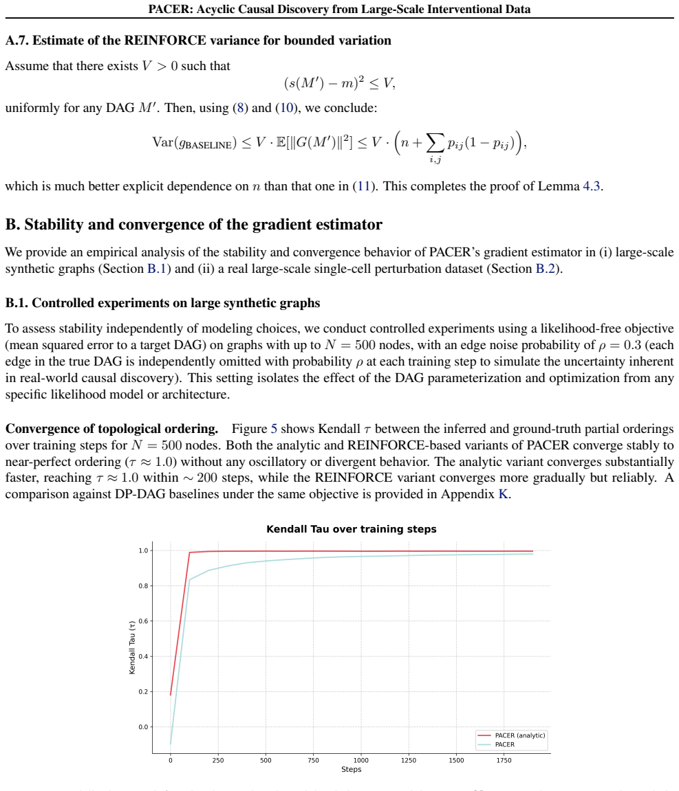
orders of magnitude larger and grows strongly with N (≈90 for N=500 vs
and increases strongly with N, confirming the critical role of the control variate. orders of magnitude larger and grows strongly with N (≈90 for N=500 vs. ≈0.002 with control variate at convergence), confirming that baseline subtraction is critical for stable large-scale training. Gradient variance across Monte Carlo samples.Figure 8 shows gradient varia...
work page 2022
-
[3]
It remains to compute the last term in equation 23, which is the variance: EM ′∼M(θ,P) h ⟨Σ−1 j (µj − ¯µj),µ j − ¯µj⟩ i =E M ′∼M(θ,P) ⟨Σ−1 j nP i=1 (aij −E[a ij])wijxi, nP i=1 (aij −E[a ij])wijxi⟩ = nP i=1 Var(aij)w2 ij⟨Σ−1 j xi,x i⟩+ nP i=1 nP k=1,k̸=i Cov(aij, akj)wijwkj ⟨Σ−1 j xi,x k⟩. To complete the proof, we use the formulas,Var(aij) =E[a ij](1−E[ai...
work page 2003
-
[4]
NOTEARS (Zheng et al., 2018), NOTEARS-LR (Fang et al., 2023), DCDI (Brouillard et al.,
sorts variables by increasing marginal variance and uses parent search to infer DAG structure. NOTEARS (Zheng et al., 2018), NOTEARS-LR (Fang et al., 2023), DCDI (Brouillard et al.,
work page 2018
-
[5]
is a method that improved stability and efficiency of DCD-based methods using an alternative acyclicity constraint. Baselines implementations.GS, GES, GIES, IAMB, MMPC, GRaSP, BOSS, and LiNGAM are benchmarked using the implementation of the Causal Discovery Toolbox (Kalainathan et al., 2020). We use the original implementation of NO-TEARS (Zheng et al., 2...
work page 2020
-
[6]
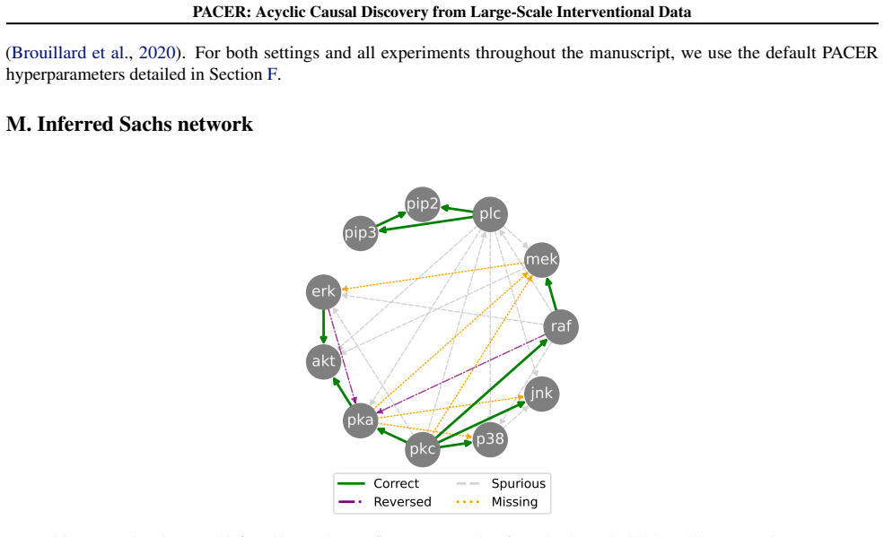
protein signaling dataset, a curated ground-truth causal graph is available. We therefore use standard structure recovery metrics that directly compare the inferred graph to the ground truth: • Structural Hamming Distance (SHD).SHD counts the minimum number of edge additions, deletions, and reversals required to transform the inferred graph into the groun...
work page 2015
-
[7]
Error bars indicate the standard deviation over three random datasets
Lower values are better for SHD, while higher values are better for precision, and recall. Error bars indicate the standard deviation over three random datasets. Table 7.Results for linear dataset with perfect interventions. Lower SHD and SID indicate better performance. Best scores are bolded and second best scores are underlined. Method 10 nodes,e=110 n...
work page 2022
-
[8]
The dataset contains 7467 measurements across 11 proteins
data from causallearn (Zheng et al., 2024). The dataset contains 7467 measurements across 11 proteins. GS, GES, GIES, IAMB, MMPC, GRaSP, BOSS, and LiNGAM are benchmarked using the implementation of the Causal Discovery Toolbox (Kalainathan et al.,
work page 2024
-
[9]
We use the original implementation of NO-TEARS (Zheng et al., 2018)
with default parameters. We use the original implementation of NO-TEARS (Zheng et al., 2018). In terms of the interventional scenario, we use the (Sachs et al.,
work page 2018
-
[10]
data processed by DCDI (Brouillard et al., 2020), containing 5846 measurements for the same 11 proteins across 6 interventional regimes. We use the IGSP, GIES, CAM, DCDI-G, and DCDI-DSF results from Appendix C1 of DCDI 36 PACER: Acyclic Causal Discovery from Large-Scale Interventional Data (Brouillard et al., 2020). For both settings and all experiments t...
work page 2020
-
[11]
comprises gene expression profiles from 218,331 melanoma cells subjected to CRISPR-based perturbations targeting 248 genes. The data was generated to identify gene regulatory programs underlying resistance or sensitivity to T cell-mediated killing, with the goal of uncovering potential therapeutic targets in cancer. We treat the three experimental conditi...
work page 2022
-
[12]
We introduce per-regime conditional parameters Ω(r) j for each intervened node j∈ I r, and include those nodes 38 PACER: Acyclic Causal Discovery from Large-Scale Interventional Data in the likelihood sum: fsoft(M ′,Ω,{Ω (r)}) = RX r=1 EX∼P (r) data "X j /∈Ir logp j Ω(Xj |M ′ j, X−j) + X j∈Ir logp j Ω(r) j (Xj |M ′ j, X−j) # . This places soft interventio...
work page 2020
discussion (0)
Sign in with ORCID, Apple, or X to comment. Anyone can read and Pith papers without signing in.