REVIEW 4 major objections 5 minor 46 references
A multi-round warm-start QAOA protocol improves Pareto-front hypervolume over single-pass weighted-sum QAOA under matched shot budgets across three benchmark stages.
Reviewed by Pith at T0; open to challenge. T0 means a machine referee read the full paper against a public rubric. the ladder, T0–T4 →
T0 review · deepseek-v4-flash
2026-08-01 14:08 UTC pith:ARXP3TOO
load-bearing objection A plausible modular multi-round QAOA framework for multi-objective optimization, but the headline gain may ride on an MPS truncation artifact and in-sample model selection. the 4 major comments →
Quantum-Enhanced Multi-Objective Optimization
The pith
A machine-rendered reading of the paper's core claim, the machinery that carries it, and where it could break.
Core claim
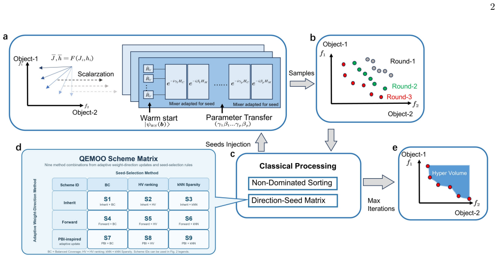
The paper's central claim is that a fixed quantum sampling budget buys a higher-quality Pareto approximation when it is distributed over multiple feedback rounds rather than spent in one pass. After an initial cold-start round of QAOA sampling over a pool of weight directions, non-dominated sorting selects elite bitstrings; a seed-selection rule (Balanced Coverage, hypervolume-ranking, or kNN sparsity) picks warm-start seeds, and an adaptive weight-direction rule (Inherit, Forward, or a PBI-inspired local linearization) generates the scalarized target for the next round. The same transferred QAOA angles are reused across all rounds; only the initial state bias changes. Under a fixed total bu
What carries the argument
The central mechanism is the multi-round feedback loop: a Direction-Seed Matrix pairs an adaptive weight-direction method with a seed-selection method, yielding nine schemes (S1–S9). The load-bearing component is the warm-start QAOA circuit that interpolates between the uniform superposition and a product state biased toward an elite seed (Eq. 9), with a rotated mixer (Eq. 10) that keeps the biased state as a fixed point; combined with transferred QAOA angles (depth p=3, trained on q_target=2 instances), this converts earlier elites into sampling priors at no additional variational cost. For strong-conflict regimes, the PBI-inspired update locally linearizes the non-linear PBI scalarization
Load-bearing premise
The framework assumes the pre-computed QAOA angles stay near-optimal for every problem size and every weight direction even though it never retunes them per instance or per direction; if that transfer assumption degrades, the benchmark compares two mistuned samplers and the reported gains would not transfer to hardware or other problem classes.
What would settle it
Fix the shot budget and compare QEMOO against a version that re-optimizes (or per-direction rescales) the QAOA angles on the n=42 Grid Large instances at the same total shot count; if per-instance angle optimization closes the hypervolume gap or reverses the ranking, the multi-round feedback gain is an artifact of a mistuned single-pass baseline. A concrete run: same weight pool, same 50,000 shots, compare transferred-angle QEMOO with angle-optimized QEMOO and angle-optimized single-pass QAOA, and report final hypervolume.
If this is right
- Under a fixed 50,000-shot budget, the best QEMOO scheme improves mean hypervolume over the single-pass weighted-sum QAOA baseline on every instance in all three benchmark stages (10/10 positive cases per stage).
- Replacing the QAOA sampler with uniformly random bitstrings at matched budget causes a large drop in front quality, so the gain is not solely from the classical selection logic.
- The dominant adaptive direction rule is stage-dependent: the PBI-inspired update dominates the strongly conflicting benchmark, while Inherit and Forward rules stay competitive on the grid benchmarks.
- The warm-start advantage is largest at the smallest per-weight budget tested (1,000 shots) and shrinks at 5,000 shots, suggesting the protocol is most valuable in shot-constrained settings.
Where Pith is reading between the lines
- Because the QAOA angles are never retuned per direction or per instance, a natural extension is to test whether per-direction angle optimization at the same shot budget closes the gap; if it does, the framework's gains reflect a mistuned baseline rather than a fundamentally better search.
- The PBI-inspired 'linearize around the elite' trick is not specific to PBI: the same local-gradient construction could synthesize effective directions for other non-linear scalarizations (e.g., Chebyshev), extending geometry-aware updates to any QAOA workflow.
- The appendix's weight-pool analysis suggests that the choice of weight distribution trades off absolute final quality against warm-start amplification; one untested design axis is to choose the pool specifically to maximize round-over-round gains.
- A hardware prediction follows from the rotated-mixer warm start: since the extra gates are single-qubit, the scheme's overhead on real devices is small, but whether the transferred angles remain near-optimal under noise is untested and would decide the practical value.
Editorial analysis
A structured set of objections, weighed in public.
Referee Report
Summary. QEMOO is presented as a multi-round, budget-matched extension of weighted-sum QAOA for multi-objective Ising problems. It splits a fixed shot budget into three rounds, uses elite seeds from non-dominated sorting to construct warm-start QAOA circuits, and couples this with three direction-update rules (Inherit, Forward, and PBI-inspired local linearization) and three seed selectors. The main evidence is an empirical comparison on three Ising benchmark suites (Grid Small n=20, Strong Conflict n=18, Grid Large n=42 with MPS χ=30) against a single-pass QAMOO baseline and uniform random sampling. The reported results select a best scheme per dataset (S6, S9, S2) and claim HV improvements in all ten instances per dataset, with the largest relative gain on Grid Large. Appendices provide parameter scans and a derivation of the PBI local linearization.
Significance. The modular separation of adaptive direction updates and seed selection is conceptually useful, and the PBI linearization in Appendix F is a clear, checkable derivation. The paper also has strengths in matching total shot budgets, including random-sampling controls, per-instance gains, and code/data release. However, the empirical claims rest on deterministic single-seed runs, in-sample selection of the best of several schemes, and a tensor-network backend with fixed bond dimension for the largest and most important gain. These issues currently prevent me from treating the 'across three benchmark stages' claim as established, although they are addressable with additional reruns and analyses.
major comments (4)
- [Sec. IV.D and Tables I-III] All experiments use fixed random seeds, so the reported means over 10 instances are single deterministic trajectories and 'positive cases 10/10' is not a statistical win rate. No confidence intervals or hypothesis tests are given. Please rerun with multiple random seeds/weight-pool draws and report paired confidence intervals and tests (e.g., Wilcoxon across instances and seeds). Without this, one cannot separate systematic improvement from seed luck.
- [Sec. V.B-V.D and Fig. 2] The headline schemes S6/S9/S2 are chosen as the best among the evaluated combinations on the same datasets used for the final tables; the manuscript itself describes a 'rerun benchmark' with stage-appropriate rows. No multiplicity control or holdout validation is applied. Since the abstract claims QEMOO 'improves' HV, please report the distribution over all schemes, or a pre-registered/holdout choice, or at least adjusted comparisons.
- [Sec. IV.D, Table III, App. C.2] The Grid-Large result is evaluated with mqmps at χ=30 on n=42; a vertical cut of the 6x7 grid requires up to χ=64 for exact representation. Warm-start and standard QAOA states can have different entanglement, so a fixed χ can differentially truncate baseline vs QEMOO. App. C.2 reports only final HV stability, not the baseline-vs-QEMOO gap or discarded weight. The largest single gain (7.5% on Grid Large) is on this backend, so the internal validity of the central claim depends on ruling out a truncation artifact. Please report ΔHV and per-scheme discarded weight vs χ (including χ=64 or larger if feasible).
- [Sec. II.C and IV.B] Transferred p=3 angles from q_target=2 are used for all directions and sizes without checking their quality on the scalarized Hamiltonians. If the transferred angles are far from optimal on n=20/18/42, the comparison may be between two variants of an ineffective sampler; this would not change the relative conclusion but would undermine the title-level 'quantum-enhanced' claim and transferability. Please provide a sanity check, e.g., approximation ratio or energy of the transferred-angle QAOA vs classically optimized angles on a few representative scalarized instances.
minor comments (5)
- [Throughout] Typos and spacing errors: 'perplayers' in Sec. II.C; 'can offers' in the first paragraph; 'aQuantum' in the contribution list; 'researchs' in Sec. I.
- [Appendix E, Table V] Table V uses normalized HV values around 1.04/0.98, while main-text tables report raw HV (e.g., 10.94e9 for Grid Large). Please clarify the normalization and state which dataset the table refers to.
- [References] References [12] and [35] appear to be the same paper (Farhi, Goldstone, Gutmann, and Zhou, Quantum 6, 759 (2022)); please consolidate.
- [Fig. 2 caption] The caption's definition of 'HV_best' and the '+1' offset is hard to parse; please specify whether HV_best is the stage-best mean HV and why the offset is used.
- [Sec. III.C] The phrase 'a cap of d_max seeds per weight direction' is ambiguous; it should be 'at most d_max seeds assigned to the same parent weight direction'.
Circularity Check
Headline HV gains are in-sample best-of-scheme/hyperparameter selections: the winning QEMOO scheme (S6/S9/S2) and Grid-Large settings (c=0.4, χ=30) are chosen from the same benchmark data used to report the gains, so the central empirical claim is partly selected rather than independently predicted.
specific steps
-
fitted input called prediction
[Sec. V.A (Fig. 2), Tables I–III; scheme selection described in Sec. IV.B]
"the plot keeps only the single best QEMOO scheme from the rerun benchmark ... Specifically, the displayed QEMOO schemes are S6 for DataSet 1: Grid Small, S9 for DataSet 2: Strong Conflict, and S2 for DataSet 3: Grid Large."
S6, S9, and S2 are not fixed methods chosen before evaluation; they are the highest-HV entries among the S1–S9 method grid scored on the same datasets (Sec. IV.B and App. A heatmaps). The headline gains and the 10/10 positive-case counts in Tables I–III are then reported for those post-hoc winners. Thus the central empirical claim 'QEMOO improves across three benchmark stages' is a max over in-sample configurations: the scheme identity is read from the same HV outcomes that serve as evidence, so the reported advantage is partly constructed by selection rather than independently predicted.
-
fitted input called prediction
[Appendix C.1/C.2, Sec. IV.D, Sec. V.D, Table III]
"the resulting Hypervolume follows a clear unimodal distribution peaking at c≈0.4 ... the highest final mean HV appearing near the latest χ=30 rerun setting ... the main Grid-Large rerun uses bond dimension χ=30."
The Grid-Large headline result (S2, mean gain 7.64e8, Table III) is produced with c=0.4 and χ=30, the hyperparameter values identified by HV scans performed on the same Grid-Large benchmark (App. C.1/C.2; App. B fixes 'the Grid-Large setting ... χ=30, and c=0.4'). Therefore the main-text Grid-Large gain is reported for hyperparameters optimized on the evaluation data itself; the appendix 'stability' scans are refits on the same data, not out-of-sample validation. The paper's own limitation statement—'settings such as χ=30, c=0.4 ... are the strongest tested choices in our benchmark suite, not universal optima'—confirms this in-sample status.
full rationale
The mathematical derivation chain is not inherently circular: Appendix F gives a genuine first-order linearization of PBI and shows how λeff maps back to a two-body Ising Hamiltonian; parameter transfer is cited to the external result [16]; warm-starting is cited to the external result [40]; and the random-sampling control is a matched control rather than a fitted outcome. However, the paper's strongest empirical conclusion—that QEMOO improves Pareto-front hypervolume across three benchmark stages—relies on stage winners S6/S9/S2 being selected as the best of the compared schemes on the same datasets used for the headline tables, and on c=0.4 and χ=30 being chosen from Grid-Large HV scans before being reused in the Grid-Large main result. This is in-sample model selection: the 'best' configuration and the reported gain come from the same evaluation, so the headline numbers are partially selected rather than independent predictions. The MPS χ=30 truncation concern raised externally is a serious internal-validity threat for the Grid-Large and quantum-vs-random evidence, but it is an experimental artifact concern, not a definitional circularity, so it does not by itself raise the circularity score. No load-bearing self-citation chain was found. Overall, the core derivation is self-contained, but the central empirical claim is partly fitted, warranting a partial-circularity score of 6 rather than 0.
Axiom & Free-Parameter Ledger
free parameters (6)
- Warm-start bias coefficient c =
0.4
- MPS bond dimension chi =
30
- PBI penalty theta_p =
not reported
- Forward deformation eta =
not reported
- Shot schedule (s1,s2,s3) =
(300,100,100)
- BC separation threshold tau and kNN k =
not reported
axioms (6)
- domain assumption QAOA parameters optimized on 2-qubit instances transfer to all n<=42 scalarized subproblems at depth p=3
- ad hoc to paper The local linearization lambda_eff = u + theta_p d2/||d2|| preserves the ability of PBI-style scalarization to target useful trade-off regions
- domain assumption MPS with bond dimension chi=30 faithfully reproduces exact QAOA output statistics and HV differences at n=42
- standard math Weighted-sum scalarization of multi-objective Ising Hamiltonians yields a single Ising Hamiltonian with projected couplings and fields
- domain assumption Hypervolume with fixed raw-energy reference points is an appropriate comparable measure across different instance scales
- domain assumption Fixed random seed 2026 is representative; results would not change qualitatively under other seeds
read the original abstract
Multi-objective combinatorial optimization requires identifying Pareto-optimal trade-off solutions among conflicting objectives, often making it more demanding than its single-objective counterpart. Although quantum multi-objective optimization methods have begun to emerge, most existing quantum optimization workflows are still built around single-objective or fixed-scalarization settings. Building on existing weighted-sum QAOA approaches to quantum multi-objective optimization, we propose QEMOO, a quantum-enhanced multi-objective optimization framework that combines Pareto-based selection and warm-started QAOA sampling in a multi-round protocol under the same total shot budget. We further introduce a PBI-inspired adaptive direction-update scheme to improve coverage in strongly conflicting benchmark regimes. Across three benchmark stages, QEMOO improves Pareto-front hypervolume over the single-pass weighted-sum QAOA baseline under matched shot budgets, suggesting a practical route toward shot-efficient quantum-assisted multi-objective optimization and its future applications.
Figures


Reference graph
Works this paper leans on
-
[1]
Ehrgott,Multicriteria Optimization, 2nd ed
M. Ehrgott,Multicriteria Optimization, 2nd ed. (Springer, 2005)
2005
-
[2]
•Whenc→1:θ q →π·b q, preparing a state close to the computational basis state|b⟩(greedy exploita- tion)
=π/2 for allq, recovering|+⟩ ⊗n (standard QAOA). •Whenc→1:θ q →π·b q, preparing a state close to the computational basis state|b⟩(greedy exploita- tion). The mixing Hamiltonian must also be adapted to pre- serve the biased initial state as a fixed point. Follow- ing [40], we replace the standardR X (2β) mixer with a rotatedmixer: U (warm) M (β) = nY q=1 R...
2026
-
[3]
Aguilera, R
E. Aguilera, R. de Santiago, B. L´ opez-Prado, C. Motz, and G. Olague, Mathematics12, 1291 (2024)
2024
-
[4]
hijacking
Repeat Steps 2–3 until allRrounds are complete. This design introduces afeedback loop: each round’s non-dominated front informs the next round’s initial quantum states, enabling adaptive reallocation of quan- tum resources toward the most promising regions of ob- jective space. B. Adaptive W eight-Direction Strategies The first design axis of QEMOO is the...
- [5]
-
[6]
P. Xu, Y. Ma, W. Lu, M. Li, W. Zhao, and Z. Dai, Jour- nal of Materials Informatics5(2025)
2025
-
[7]
J. R. Figueira, C. M. Fonseca, P. Halffmann, K. Klam- roth, L. Paquete, S. Ruzika, B. Schulze, M. Stiglmayr, and D. Willems, Technical Report (2016)
2016
-
[8]
K. Deb, A. Pratap, S. Agarwal, and T. Meyarivan, IEEE Transactions on Evolutionary Computation6, 182 (2002)
2002
-
[9]
Zhang and H
Q. Zhang and H. Li, IEEE Transactions on Evolutionary Computation11, 712 (2007)
2007
-
[10]
Boland, H
N. Boland, H. Charkhgard, and M. Savelsbergh, Euro- pean journal of operational research260, 904 (2017)
2017
-
[11]
D¨ achert, T
K. D¨ achert, T. Fleuren, and K. Klamroth, Mathematical Methods of Operations Research100, 351 (2024)
2024
-
[12]
E. Farhi, J. Goldstone, and S. Gutmann, arXiv preprint arXiv:1411.4028 (2014)
Pith/arXiv arXiv 2014
-
[13]
M. P. Harrigan, K. J. Sung, M. Neeley, K. J. Satzinger, F. Arute, K. Arya, R. Babbush, D. Bacon, J. C. Bardin, R. Barends,et al., Nature Physics17, 332 (2021)
2021
-
[15]
S. Boulebnane, A. Khan, M. Liu, J. Larson, D. Herman, R. Shaydulin, and M. Pistoia, Evidence that the quan- tum approximate optimization algorithm optimizes the sherrington-kirkpatrick model efficiently in the average case (2025), arXiv:2505.07929 [quant-ph]
Pith/arXiv arXiv 2025
-
[16]
D. Lykov, J. Wurtz, C. Poole, M. Saffman, T. Noel, and Y. Alexeev, npj Quantum Information9, 10.1038/s41534-023-00718-4 (2023)
-
[17]
R. Shaydulin, C. Li, S. Chakrabarti, M. DeCross, D. Her- man, N. Kumar, J. Larson, D. Lykov, P. Minssen, Y. Sun, Y. Alexeev, J. M. Dreiling, J. P. Gaebler, T. M. Gatter- man, J. A. Gerber, K. Gilmore, D. Gresh, N. Hewitt, C. V. Horst, S. Hu, J. Johansen, M. Matheny, T. Men- gle, M. Mills, S. A. Moses, B. Neyenhuis, P. Siegfried, R. Yalovetzky, and M. Pist...
-
[18]
S. H. Sureshbabu, D. Herman, R. Shaydulin, J. Basso, S. Chakrabarti, Y. Sun, and M. Pistoia, Quantum8, 1231 (2024)
2024
-
[19]
Shaydulin, S
R. Shaydulin, S. Hadfield, T. Hogg, and M. Pistoia, ACM Transactions on Quantum Computing4, 1 (2023)
2023
-
[20]
X. Zhu, Z. Zou, F. Jin, P. Mosharev, M. Luo, Y. Wu, J. Chen, C. Zhang, Y. Gao, N. Wang, Y. Zou, A. Zhang, F. Shen, Z. Bao, Z. Zhu, J. Zhong, Z. Cui, Y. Han, Y. He, H. Wang, J.-N. Yang, Y. Wang, J. Shen, G. Liu, Z. Song, J. Deng, H. Dong, P. Zhang, C. Song, Z. Wang, H. Li, Q. Guo, M.-H. Yung, and H. Wang, National Science Review 10.1093/nsr/nwag124 (2026)
-
[21]
P. Chandarana, S. V. Romero, A. G. Cadavid, A. Simen, E. Solano, and N. N. Hegade, Hybrid sequential quantum computing (2025), arXiv:2510.05851 [quant-ph]
arXiv 2025
-
[22]
Kotil, A
A. Kotil, A. Banerjee, S. Ghosh, A. Yakaryilmaz, D. Her- man, S. H. Sureshbabu, R. Shaydulin, Y. Sun, M. Pis- toia, and S. Chakrabarti, Nature Computational Science , 1 (2025)
2025
-
[23]
Das and J
I. Das and J. E. Dennis, SIAM Journal on Optimization 8, 631 (1998)
1998
-
[24]
Ekstr¨ om, H
L. Ekstr¨ om, H. Wang, and S. Schmitt, Physical Review Research7, 023141 (2025)
2025
-
[25]
L. Ekstrøm, H. Wang, S. Schmitt, and N. Awasthi, arXiv preprint arXiv:2602.10952 (2026)
arXiv 2026
-
[26]
A. D. King, arXiv preprint arXiv:2511.01762 (2025)
arXiv 2025
-
[27]
Ayodele, R
M. Ayodele, R. Allmendinger, M. L´ opez-Ib´ a˜ nez, and M. Parizy, inOperations Research Proceedings 2022, Lec- ture Notes in Operations Research, edited by O. Grothe, S. Nickel, S. Rebennack, and O. Stein (Springer Nature Netherlands, 2023) pp. 393–399
2022
-
[28]
Schworm, X
P. Schworm, X. Wu, M. Klar, M. Glatt, and J. C. Aurich, Journal of Manufacturing Systems72, 142 (2024)
2024
-
[29]
Sawamura, K
K. Sawamura, K. Araki, N. Maruyama, R. Haba, and M. Ohzeki, Journal of the Physical Society of Japan95, 054002 (2026)
2026
-
[30]
Zitzler, L
E. Zitzler, L. Thiele, M. Laumanns, C. M. Fonseca, and V. G. da Fonseca, IEEE Transactions on Evolutionary Computation7, 117 (2003)
2003
-
[31]
C. M. Fonseca, L. Paquete, and M. L´ opez-Ib´ a˜ nez, in IEEE Congress on Evolutionary Computation(2006) pp. 1157–1163
2006
-
[32]
Riquelme, C
N. Riquelme, C. Von L¨ ucken, and B. Baran, inLatin American Computing Conference (CLEI)(2015) pp. 1– 11
2015
-
[33]
Beume, C
N. Beume, C. M. Fonseca, M. L´ opez-Ib´ a˜ nez, L. Paquete, and J. Vahrenhold, IEEE Transactions on Evolutionary Computation13, 1075 (2009)
2009
-
[34]
A. P. Guerreiro, C. M. Fonseca, and L. Paquete, ACM Computing Surveys54, 1 (2022)
2022
-
[35]
Lucas, Frontiers in Physics2, 74887 (2014)
A. Lucas, Frontiers in Physics2, 74887 (2014)
2014
-
[36]
E. Farhi, J. Goldstone, and S. Gutmann, arXiv preprint arXiv:1412.6062 (2015)
Pith/arXiv arXiv 2015
-
[37]
Farhi, J
E. Farhi, J. Goldstone, S. Gutmann, and L. Zhou, Quan- tum6, 759 (2022)
2022
-
[38]
Akshay, H
V. Akshay, H. Philathong, M. E. S. Morales, and J. D. Biamonte, Physical Review A104, 012403 (2021)
2021
- [39]
-
[40]
J. A. Monta˜ nez Barrera, D. Willsch, and K. Michielsen, arXiv preprint arXiv:2402.02833 (2024)
Pith/arXiv arXiv 2024
-
[41]
A. Galda, X. Liu, D. Lyou, Y. Feng, and Y. Alexeev, arXiv preprint arXiv:2106.07531 (2021)
Pith/arXiv arXiv 2021
-
[42]
D. J. Egger, J. Mareˇ cek, and S. Woerner, Quantum5, 479 (2021)
2021
-
[43]
Biscani and D
F. Biscani and D. Izzo, Journal of Open Source Software 5, 2338 (2020)
2020
-
[44]
smoother is always better
MindQuantum Developer, Mindquantum, version 0.6.0, https://gitee.com/mindspore/mindquantum(2021), a hybrid quantum-classical framework. Appendix A: F ull Heatmaps of Method Combinations For completeness, we provide the full comparison of stage-wise method combinations for the rerun raw-HV bench- mark. This appendix is the detailed counterpart of the main-...
2021
-
[45]
We explore its impact by scanning fromc= 0.1 (weak bias) toc= 0.8 (strong exploitation) across all test instances
Selection Strategy for Mixing Coefficientc The warm-start bias coefficientc∈[0,1] serves as the primary control for the exploration–exploitation trade-off. We explore its impact by scanning fromc= 0.1 (weak bias) toc= 0.8 (strong exploitation) across all test instances. As shown in Figure 8, the resulting Hypervolume follows a clear unimodal distribution ...
-
[46]
The left panel in Fig
Bond-Dimension Scaling for the Best Large-MPS Case To assess how tensor-network approximation quality interacts with the best Grid-Large configuration, we vary the bond dimensionχwhile keeping the same warm-start protocol and best observed direction policy. The left panel in Fig. 9 shows the HV-vs-shots trajectories for differentχvalues, and the right pan...
-
[47]
The left panel in Fig
W eight-Count Scaling for the Best Large-MPS Case To complement the warm-start coefficient analysis, we also examine how the best Grid-Large configuration changes as the number of sampled weights varies while keeping the same transferred parameters and sampling protocol. The left panel in Fig. 10 shows the HV-vs-shots trajectories for different weight cou...
1925
discussion (0)
Sign in with ORCID, Apple, or X to comment. Anyone can read and Pith papers without signing in.