REVIEW 2 major objections 6 minor 25 references
Testing a Computed Tomography Imaging Spectrometer for Earth Observations on the HEIMDAL Stratospheric Balloon Mission
T0 review · 2 major / 6 minor · reviewed 2026-08-05 · deepseek-v4-flash
Pith's one-line read This paper reports the first stratospheric flight of a snapshot CTIS hyperspectral camera, with reconstructed datacubes separating land from water.
desk verdict First CTIS on a stratospheric balloon: credible engineering demonstration, but spectral fidelity claims rest on an untested system matrix assumption. read the letter →
The pith
A machine-rendered reading of the paper's core claim, the machinery that carries it, and where it could break.
The reading
What carries the argument
Computed Tomography Imaging Spectroscopy (CTIS) is the central mechanism: a 2D diffractive optical element spreads each scene point into a 3×3 diffraction pattern (a central zeroth order and eight first orders) on a 2D sensor. The measured diffraction image g is modeled as g = Hf + n, where f is the vectorized 3D datacube and H is the system matrix encoding diffraction efficiency, lens transmission, sensor response, illumination, and vignetting. Because the system is underdetermined, reconstruction uses either the EM iteration (20 iterations, initialized with Hᵀg) or a physics-guided convolutional autodecoder that includes a UNet and a second network refining the estimated CTIS image. This H
What would settle it
Image a set of calibrated reflectance panels with known spectral features using both the original and the flight outermost lens, reconstruct with the same H, and compare the recovered reflectance spectra. If the spectral shape or the position of absorption features shifts by more than the reconstruction noise, the transferability of H fails and the land/water accuracy is not evidence about the flight configuration.
Extended reading notes
Core claim
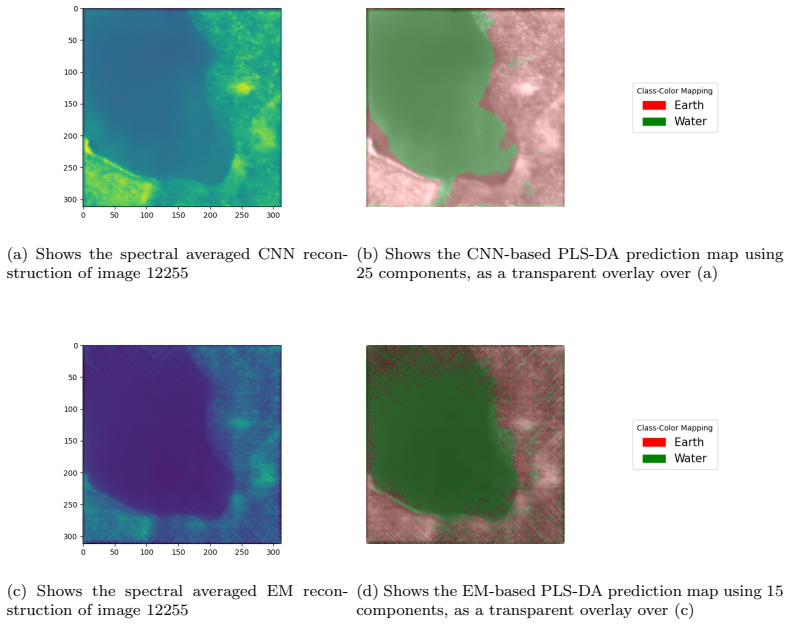
The central claim is that a CTIS snapshot hyperspectral camera—previously a lab instrument—can be made robust enough for stratospheric balloon operations and can return scientifically usable hyperspectral data. During the HEIMDAL flight the system survived ascent, float at about 28 km, and landing, stored all images, and reconstructed 3D datacubes (312×312 spatial pixels, 145 or 236 spectral channels). A proof-of-principle analysis selected 23 images containing land and water, masked the two classes, and trained PLS-DA classifiers on 5×5 averaged, SNV-normalized spectra; the CNN-reconstructed cubes supported land/water discrimination at about 0.8 cross-validation accuracy versus 0.58 for EM
Load-bearing premise
The measurement model H was built for a nearly identical camera with a different outermost lens and is used unchanged for the flight camera; if that lens alters how light is collected or vignetted, every reconstructed datacube and the classification built on it could be systematically distorted.
Editorial extensions
If this is right
- Balloon platforms gain a motion-robust hyperspectral mode: 4–10 ms snapshot exposures avoid the smearing that pushbroom scanners suffer from gondola rotation and pendular swings.
- Reconstructed datacubes can be produced on board during flight (every tenth image), so a downlink-limited balloon can still monitor what the camera sees near real time.
- Land/water discrimination from reconstructed spectra shows that CTIS data are informative enough for a first land-cover classification, at about 0.8 accuracy with CNN reconstruction.
- At roughly 3.4 m ground sampling distance from 26 km, the platform sits in the resolution range needed to resolve individual tree crowns, motivating future tree-type classification.
- Thermal and power margins were validated: the payload survived a five-hour flight with insulated electronics and dual battery packs, so the approach can be repeated.
Reading between the lines
- The paper carries the system matrix H over from an earlier optical configuration that differs in the outermost lens; if that lens changes the diffraction pattern or vignetting, the reconstructed spectra—and the 0.8 accuracy—could partly reflect artifacts. A re-calibration with the flight lens would settle this.
- CNN reconstruction beating EM by 0.22 in accuracy may indicate that the network has learned to compensate for H mismatch or noise; comparing both reconstructions against a field spectrometer over known targets would separate recovered physics from learned priors.
- The blurred waterline in the prediction maps hints that the 600–850 nm window sees water-column or mixed-pixel effects; extension to aquatic or wetland classification would require sunglint modeling or spectral unmixing, which the paper does not do.
- The spectral spacing implied by 145–236 channels over 600–850 nm is fine enough for chlorophyll absorption features, so tree-species classification is a plausible next step once the H-matrix transferability question is resolved.
Signed reviews
Editorial analysis
A structured set of objections, weighed in public.
Referee Report
Summary. The paper reports the development and test of a snapshot hyperspectral imager based on Computed Tomography Imaging Spectroscopy (CTIS) for stratospheric balloon Earth observation. The payload was environmentally tested in a thermal-vacuum chamber and flown on the 5.5-hour HEIMDAL BEXUS balloon mission from Esrange in October 2024. Raw CTIS diffraction images were acquired at 1 FPS and stored; datacubes were reconstructed both on-board and post-flight using CNN- and EM-based algorithms built on a system matrix taken from prior work. A proof-of-principle PLS-DA analysis is used to distinguish land and water from reconstructed spectra, with reported cross-validation accuracy of about 0.8 for CNN and 0.58 for EM reconstructions. The central claim is that this is the first stratospheric HAB flight of a CTIS snapshot hyperspectral camera and that usable hyperspectral data were obtained.
Significance. If the reconstruction chain is valid, the paper provides a valuable first demonstration of CTIS snapshot hyperspectral imaging from a stratospheric balloon, an important complement to pushbroom systems that are motion-sensitive. The mission integration details—mechanical design, power system, thermal-vacuum testing, on-board storage and reconstruction, and data recovery—are useful engineering references for the HAB community. The authors are transparent about operational issues such as RGB underexposure and late-flight condensation. However, the quantitative support for the 'usable hyperspectral data' claim rests on an unvalidated reuse of a system matrix from a previous optical configuration, and the classification demonstration is statistically underreported.
major comments (2)
- [Sec. 2.3 / Eq. (1)] The entire reconstruction chain rests on the system matrix H from the authors' prior work [10]. Section 2.1 states that the flight camera uses the same optical system as [10] 'with the sole exception of the outermost lens,' and Sec. 2.3 then says that the [10] H construction applies. Since H encodes dispersion scale, vignetting, and point-spread function, a change in the outer lens can systematically bias every reconstructed datacube and therefore the land/water classification. No calibration validation under the flight lens configuration is reported—e.g., a monochromatic source imaged through the flight optics, comparison of measured versus predicted 3×3 diffraction-order positions/widths, or a known reflectance target. Please add such a calibration check, or explicitly state that the H-matrix assumption is an unvalidated approximation and downgrade the quantitative spectral claims acco
- [Sec. 5.2 / Figs. 13–15] The PLS-DA accuracy values (0.8 CNN, 0.58 EM) are reported without error bars, cross-validation details (number of folds, repeated CV), or an independent test set. The training data consist of 23 manually selected/masked datacubes with a 72/28 land/water imbalance. The claim that the CNN-based model 'will outperform' the EM-based model is not statistically supported as presented. Please report the CV protocol, per-class accuracy/precision/recall, and confidence intervals, or recast the comparison as qualitative rather than quantitative.
minor comments (6)
- [Sec. 2.3] The in-text citation 'Eq. 2.3' should refer to Eq. (1). Also, in Eq. (2) the denominator notation 'Pq2 i=1 Hij' is unclear; please define the row-sum operation and state the dimensions explicitly.
- [Sec. 5.2 / Fig. 13] The y-axis of Fig. 13 is labeled 'R-squared values' while the text calls the metric 'accuracy'; please clarify which quantity is plotted and how it is computed for a classification problem.
- [Sec. 2.2] Please explain why the number of spectral channels differs between CNN (236) and EM (145) reconstructions; the current text merely states the numbers without a reason.
- [Abstract / Sec. 3.2] The abstract describes the system as 'able to record near-video-rate images,' but the flight acquisition rate was 1 image/s. Please specify the actual rate in the abstract or provide bench evidence for higher-rate operation.
- [Sec. 3.2] The statement that ~2000 datacubes were reconstructed on-board is not accompanied by which algorithm (CNN, EM, or both), what parameters were used, or whether those cubes were validated against post-flight reconstructions. Please clarify.
- [Various] The text contains typos and minor inconsistencies: 'wavelenght' (Sec. 2.2), 'traind' (Fig. 15 caption), 'ballon' (Sec. 3), inconsistent use of 'datacube' vs 'data cube', and reference [20] contains an 'accessed: [date]' placeholder. A careful proofread is recommended.
Circularity Check
No circular derivation: H-matrix reuse is calibration, not circularity; PLS-DA is cross-validated analysis, not a fitted prediction.
full rationale
The paper's central claims are empirical demonstrations: acquiring CTIS images in simulated stratospheric conditions and on the HEIMDAL HAB flight, reconstructing datacubes, and performing land/water discrimination. None of these reduce to a fitted parameter or self-referential definition. Eq. (1), g = Hf + n, is a standard linear imaging model, and H is a calibration matrix whose construction is imported from the authors' prior work [10] (Sec. 2.3: 'the optical system of the CTIS cameras is the same ... as the system outlined in [10], which also applies to the construction of the H matrix'). This is a reuse of an independently calibrated quantity, not a self-definitional loop: H is not defined in terms of the flight datacubes or the PLS-DA labels, and it is falsifiable by external calibration measurements. The CNN/EM reconstructions are inverse estimation algorithms applied to measured diffraction images; the paper does not claim to 'predict' the reconstructions from H alone. The PLS-DA models are trained on manually masked spectra from 23 reconstructed datacubes and evaluated via cross-validation accuracy (Fig. 13); this is a standard supervised analysis of acquired data, not a fitted parameter renamed as a prediction. The only notable weakness is the unvalidated assumption that H remains valid after the outer lens change: Sec. 2.1 states the outer 50 mm lens 'effectively determin[es] the focal length', while Sec. 2.3 states the system is identical to [10] 'with the sole exception of the outermost lens'. That is a correctness/validation gap, not circularity, because it does not make the output equal to the input by construction. No uniqueness theorems, ansatz-smuggling citations, or renaming of known results are load-bearing. Score 0.
Assumptions & free parameters
free parameters (4)
- PLS-DA component count (CNN) =
25
- PLS-DA component count (EM) =
15
- EM reconstruction iterations =
20
- Number of manually selected training datacubes =
23
assumptions (5)
- domain assumption Linear imaging equation g = Hf + n holds with known system matrix H
- domain assumption The H matrix calibrated in [10] remains valid for the HAB configuration with a different outermost lens
- standard math EM algorithm converges in 20 iterations to a meaningful inverse of the underdetermined system
- ad hoc to paper PLS-DA on SNV-normalized 5x5 averaged spectra can distinguish land and water
- domain assumption Atmospheric path radiance and scattering do not dominate the spectral differences between land and water
Cite this review
Pith. "Pith review of Testing a Computed Tomography Imaging Spectrometer for Earth Observations on the HEIMDAL Stratospheric Balloon Mission." pith.science (2026). https://pith.science/paper/AUILOTK2
@misc{pith2026250819693,
  author       = {Pith},
  title        = {Pith review of: Testing a Computed Tomography Imaging Spectrometer for Earth Observations on the HEIMDAL Stratospheric Balloon Mission},
  year         = {2026},
  howpublished = {\url{https://pith.science/paper/AUILOTK2}},
  note         = {Machine review of arXiv:2508.19693}
}
read the original abstract
Stratospheric High Altitude Balloons (HABs) have great potential as a remote sensing platform for Earth Observations that complements orbiting satellites and low flying drones. At altitudes between 20-35 kms, HABs operate significantly closer to ground than orbiting satellites, but significantly higher than most drones. HABs therefore offer a unique potential to deliver high spatial resolution imaging with large area coverage. Another two imaging parameters that are important for Earth Observation applications are spectral resolution and spectral range. In this paper, we therefore present the development and testing of a hyperspectral imaging system, able to record near-video-rate images in narrow contiguous spectral bands, from a HAB platform. In particular, we present the first stratospheric environmental tests and HAB flight of a snapshot hyperspectral camera, based on Computed Tomography Imaging Spectroscopy (CTIS), which is well suited to cope with the challenges posed by the motion of the HAB platform and the stratospheric environment. We have successfully acquired images with the system under both simulated stratospheric conditions in the Mars Simulation Laboratory at Aarhus University and during a 5 hour HAB flight mission named HEIMDAL from Kiruna in October 2024 as part of the REXUS/BEXUS 34/35 2024 campaign organized by DLR-SNSA. The study represents a step towards deploying the HAB platform for high quality land cover classification.
Figures


Figures from the paper (14 more)





Reference graph
Works this paper leans on
-
[10]
M. Ahlebæk, M. Peters, W.-C. Huang, M. Frandsen, R. Erik- sen, B. Jørgensen, The hybrid approach—convolutional neural net- works and expectation maximisation algorithm—for tomographic re- construction of hyperspectral images, J. Spectral Imaging (2023) a1doi:10.1255/jsi.2023.a1
-
[1]
Floberghagen, Why HAPS for EO, HAPS4ESA (2024)
R. Floberghagen, Why HAPS for EO, HAPS4ESA (2024). URL https://atpi.eventsair.com/haps4esa2024/
work page 2024
-
[2]
A. Pankine, Z. Li, D. Parsons, M. Purucker, E. Weinstock, W. Wis- combe, K. Nock, Stratospheric satellites for earth observations, Bulletin of The American Meteorological Society - BULL AMER METEOROL SOC 90 (08 2009). doi:10.1175/2009BAMS2624.1
-
[3]
Drinkwater, FutureEO, HAPS4ESA (2019)
M. Drinkwater, FutureEO, HAPS4ESA (2019). URL https://atpi.eventsair.com/haps4esa2024/
work page 2019
- [4]
-
[5]
B. Boldrini, W. Kessler, K. Rebner, R. W. Kessler, Hyperspectral imag- ing: a review of best practice, performance and pitfalls for in-line and on-line applications, Journal of near infrared spectroscopy 20 (5) (2012) 483–508
work page 2012
-
[6]
M. Descour, E. Dereniak, Computed-tomography imaging spectrometer: experimental calibration and reconstruction results, Appl. Opt. 34 (22) (1995) 4817–4826. doi:10.1364/AO.34.004817
-
[7]
T. V. Bulygin, G. N. Vishnyakov, Spectrotomography: a new method of obtaining spectrograms of two-dimensional objects, in: G. G. Levin (Ed.), Analytical Methods for Optical Tomography, Vol. 1843, Interna- tional Society for Optics and Photonics, SPIE, 1992, pp. 315 – 322. URL https://doi.org/10.1117/12.131904
Show all 25 references
-
[8]
Okamoto, I
T. Okamoto, I. Yamaguchi, Simultaneous acquisition of spec- tral image information, Opt. Lett. 16 (16) (1991) 1277–1279. doi:10.1364/OL.16.001277
1991 doi
-
[9]
Huang, M
W.-C. Huang, M. S. Peters, M. J. Ahlebaek, M. T. Frandsen, R. L. Eriksen, B. Jørgensen, The application of convolutional neural networks for tomographic reconstruction of hyperspectral images, Displays (2022) 102218doi:10.1016/j.displa.2022.102218. 31
2022
-
[12]
M. S. Peters, M. J. Ahlebæk, M. T. Frandsen, B. Jørgensen, C. H. Jessen, A. K. Carlsen, M. S. Andersen, W.-C. Huang, R. L. Eriksen, In- vestigating the applicability of a snapshot computed tomography imag- ing spectrometer for the prediction of °brix and ph of grapes, Spec- tr...
2025
-
[13]
M¨ ayr¨ a, S
J. M¨ ayr¨ a, S. Keski-Saari, S. Kivinen, T. Tanhuanp¨ a¨ a, P. Hurskainen, P. Kullberg, L. Poikolainen, A. Viinikka, S. Tuominen, T. Kumpula, P. Vihervaara, Tree species classification from airborne hy- perspectral and lidar data using 3d convolutional neural net- works, Remo...
2021
-
[14]
Ballanti, L
L. Ballanti, L. Blesius, E. Hines, B. Kruse, Tree species classification using hyperspectral imagery: A comparison of two classifiers, Remote Sensing 8 (6) (2016). doi:10.3390/rs8060445
2016 doi
-
[15]
Masaitis, G
G. Masaitis, G. Mozgeris, Some peculiarities of laboratory measured hyperspectral reflectance characteristics of scots pine and norway spruce needles, Research for Rural Development 2 (2012) 25–32
2012
-
[16]
P. R. Nelson, A. J. Maguire, Z. Pierrat, E. L. Orcutt, D. Yang, S. Serbin, G. V. Frost, M. J. Macander, T. S. Magney, D. R. Thompson, J. A. Wang, S. F. Oberbauer, S. V. Zesati, S. J. Davidson, H. E. Epstein, S. Unger, P. K. E. Campbell, N. Carmon, M. Velez-Reyes, K. F. Huemm- ...
2022
-
[17]
Delaur´ e, J
B. Delaur´ e, J. Blommaert, S. Livens, D. Nuyts, G. Strackx, T. Van Achteren, High resolution hyperspectral imaging from haps, hAPS4ESA (10 2017)
2017
-
[18]
P. J. Navarro, L. Miller, M. V. D ´ ıaz-Gali´ an, A. Gila-Navarro, D. J. Aguila, M. Egea-Cortines, A novel ground truth multispectral image dataset with weight, anthocyanins, and Brix index measures of grape berries tested for its utility in machine learning pipelines, GigaSci...
2022 doi
-
[19]
M. S. Peters, R. L. Eriksen, B. Jørgensen, High-resolution snapshot hyperspectral computed tomography imaging spectrometer: real-world applications, in: Unconventional Optical Imaging III, Vol. 12136, SPIE, 2022, pp. 211–216. doi:10.1117/12.2621128
2022 doi
-
[20]
The Morton Arboretum, Norway spruce (picea abies), accessed: [date] (n.d.)
-
[21]
B. R. Parizek, K. Christianson, R. B. Alley, D. Voytenko, I. Vaˇ nkov´ a, T. H. Dixon, R. T. Walker, D. M. Holland, Ice-cliff failure via retrogres- sive slumping, Geology 47 (5) (2019) 449–452. doi:10.1130/G45880.1
2019 doi
-
[22]
White, W
L. White, W. B. Bell, R. Haygood, Accelerating computed tomo- graphic imaging spectrometer reconstruction using a parallel algo- rithm exploiting spatial shift-invariance, Opt. Eng. 59 (05) (2020) 1. doi:10.1117/1.OE.59.5.055110
2020 doi
-
[23]
Douarre, C
C. Douarre, C. Crispim-Junior, A. Gelibert, G. Germain, L. Tougne, D. Rousseau, CTIS-net: A neural network architecture for com- pressed learning based on computed tomography imaging spec- trometers, IEEE Trans. Comput. Imaging 7 (2021) 572–583. doi:10.1109/TCI.2021.3083215
2021
-
[24]
M. Mel, A. Gatto, P. Zanuttigh, Joint reconstruction and super resolu- tion of hyper-spectral ctis images., in: BMVC, 2022, p. 1063. 33
2022
-
[25]
L. Wu, W. Cai, Ctis-gan: computed tomography imaging spectrometry based on a generative adversarial network, Applied Optics 62 (03 2023). doi:10.1364/AO.478230
2023 doi
-
[26]
Zimmermann, S
M. Zimmermann, S. Amann, M. Mel, T. Haist, A. Gatto, Deep learning- based hyperspectral image reconstruction from emulated and real com- puted tomography imaging spectrometer data, Optical Engineering 61 (05 2022). doi:10.1117/1.OE.61.5.053103. 34
2022 doi
Reviewed August 5, 2026 · model on record in the stance chip above.
Discussion (0). Continue with ORCID to comment.