REVIEW 3 major objections 4 minor 60 references
Worldline-Susceptibility Scheduling for Quantum Annealing Beyond Local-Adiabatic Evolution
T0 review · 3 major / 4 minor · reviewed 2026-08-02 · deepseek-v4-flash
Pith's one-line read A worldline-susceptibility schedule, built from classical Monte Carlo during simulated quantum annealing, beats both linear and exact local-adiabatic annealing at finite time.
desk verdict A practical surrogate schedule with good engineering, but the 'beats exact Roland–Cerf' claim is undermined by a gap-only baseline that omits the transition matrix element. read the letter →
The pith
A machine-rendered reading of the paper's core claim, the machinery that carries it, and where it could break.
The reading
What carries the argument
The central object is the worldline magnetization susceptibility chi_m(s) = NM(<m^2>-<|m|>^2), computed from equilibrium Suzuki-Trotter Monte Carlo samples of the transverse-field Ising model; near criticality it scales as 1/Delta(s)^2, making it a measurable surrogate for the inverse-square gap that drives the Roland-Cerf condition. The schedule is ds/dt = 1/[T(chi_m(s)+chi_0)], which allocates time by the susceptibility's cumulative weight.
What would settle it
Recompute the Roland-Cerf schedule on the same instances including the full matrix element |<E1|partial_s H|E0>| in the velocity integral; if the surrogate no longer beats it on a substantial fraction of instances, the central claim fails. A cheaper check: evaluate the matrix element for the n=10 and n=12 instances and test whether the boundary-gap trap and oscillations persist.
Extended reading notes
Core claim
Using exact diagonalization as ground truth for Sherrington-Kirkpatrick instances (n=10-20), the authors show that a schedule constructed from the worldline magnetization susceptibility measured during SQA consistently gives the highest disorder-averaged ground-state probability, beating linear ramps and, for a large fraction of instances, the exact Roland-Cerf schedule. They attribute this to two mechanisms: the boundary-gap trap, in which the true local-adiabatic schedule concentrates runtime at s=1 where the transverse field has vanished, and an oscillatory instability, in which extreme runtime localization around an interior gap produces multilevel coherent interference. The susceptibili
Load-bearing premise
The benchmarked 'exact Roland-Cerf schedule' is built from the inverse-square gap alone, omitting the transition-matrix element |<E1|partial_s H|E0>| of the true local-adiabatic condition; if that element varies along the anneal, the schedule being outperformed is not the exact one.
Editorial extensions
If this is right
- Schedule construction no longer requires diagonalizing the quantum Hamiltonian; any problem amenable to SQA can be scheduled from the same Monte Carlo run that solves it.
- Exact spectral-gap strategies can fail at finite time in two identifiable ways, and both are avoided by smoothing the time allocation over the critical region.
- The fraction of instances exhibiting the boundary-gap trap grows with system size, so the advantage of observable-based scheduling should widen for larger problems.
- The method comes with an open-source implementation, making the schedule reproducible and directly applicable to QUBO/Ising optimization workflows.
Reading between the lines
- If the transition-matrix element in the true Roland-Cerf condition is not constant, the claimed 'exact' benchmark is a gap-only schedule; a fairer comparison might narrow the reported advantage, though it would likely preserve the surrogate's edge over linear annealing.
- The same susceptibility signal could be used to time pauses or reverse ramps in hardware annealers, since it identifies when quantum fluctuations are dynamically relevant.
- The Delta* of about 0.016 failure threshold suggests a cheap predictor: instances with minimum spectral gaps below this value are the ones where gap-based scheduling is most likely to backfire.
Editorial analysis
A structured set of objections, weighed in public.
Referee Report
Summary. This paper proposes a surrogate annealing schedule for quantum annealing constructed from the worldline magnetization susceptibility χ_m(s) measured in simulated quantum annealing. The schedule is defined by ds/dt = 1/[T(χ_m(s)+χ_0)] (Eq. 14), with cumulative mapping Eq. (11). Using exact diagonalization of Sherrington–Kirkpatrick instances (n=10–20), the authors compare the surrogate against linear annealing and the Roland–Cerf local-adiabatic schedule. They report that the surrogate achieves the highest disorder-averaged ground-state probability at all system sizes and finite times studied, and they attribute this to two finite-time failure modes of exact local-adiabatic scheduling: a boundary-gap trap and an oscillatory instability. The manuscript includes an open-source implementation (qanneal), decoherence checks under Lindblad dephasing, a Trotter-parameter robustness study, and a held-out logistic validation of a gap-based failure threshold.
Significance. If the findings hold, this is a practically relevant result: a low-cost equilibrium observable can schedule annealing better than a spectral-gap-optimal schedule at realistic finite times. The paper's strengths include the open-source framework, the use of exact diagonalization only for validation, the systematic disorder ensembles, and the supplementary checks (dephasing, Trotter refinement, held-out classification). The central empirical comparison, however, depends on the correct implementation of the exact Roland–Cerf baseline and on the validity of the proposed failure-mode explanation; both need the revisions below.
major comments (3)
- [III.C, Eq. (24); Appendix A.5] The cumulative Roland–Cerf time-allocation F(s) in Eq. (24) is defined as ∫Δ^{-2}ds'/∫Δ^{-2}ds', but the Roland–Cerf velocity in Eq. (4) contains the transition matrix element M(s)=|<E1|∂sH|E0>|. The actual cumulative allocation is F_M(s)=∫M(s')Δ^{-2}ds'/∫M(s')Δ^{-2}ds'. The paper neither shows M(s) is constant nor bounds its variation. Consequently, Fig. 5 and the quantitative statements built on it (e.g., 'half the total annealing time after s≈0.995' for the n=12 instance) are not established for the exact RC schedule. Appendix A.5 states that RC trajectories were generated from Eq. (4); hence either the figure is mislabeled as 'RC cumulative weight' or the benchmark actually used a gap-only schedule, which would invalidate the headline comparison. Please recompute the cumulative allocation with M(s), or state explicitly that F(s) is an approximation and verify the failure-mode conclus
- [III.C.2] The oscillatory instability is attributed to 'coherent multilevel interference' on the basis of (i) a period mismatch with two-level LZS (T_LZS≈312 vs T_obs≈20) and (ii) survival under dephasing up to γ=0.01 (Appendix B.1). Neither diagnostic demonstrates multilevel interference: a period mismatch could arise from other causes, and dephasing robustness shows the effect is coherent but does not identify the subspace involved. Please provide direct evidence, e.g., populations of excited eigenstates during the RC-scheduled evolution, or a comparison with a truncated few-level model. Without this, the abstract's claim to have 'demonstrated' the mechanism is too strong.
- [III.D, Figs. 7–9] At n≥14 the number of instances is 50, 50, and 20, and the plotted SEM bands appear to overlap substantially in several panels. The claim that the surrogate schedule 'consistently achieves the highest average ground-state probability' across all system sizes is not supported by a formal statistical analysis. Report pairwise differences with confidence intervals or significance tests (e.g., paired tests over instances) for surrogate vs Roland–Cerf and surrogate vs linear at each n and T. This is central to the generalization claim.
minor comments (4)
- [Appendix A.6] The text says 'Ground-state probabilities [Eq. (19) of the main text]' but the relevant definition is Eq. (20) (or Eq. 16). Please correct the cross-reference.
- [III.C] The sentence 'Although both schedules satisfy exactly the same local-adiabatic condition, they produce two qualitatively different dynamical pathologies' is confusing because the two panels of Fig. 5 show two different instances, not two different schedules. Rephrase to describe the two instances.
- [III.D and Appendix B.5] The classification of instances as boundary-gap (B), oscillatory (O), or conventional (C) is used for the base rates in Figs. 7–9 and 14, but the criteria are not defined in the main text. State the classification rule (e.g., location of s*_ED and number of direction changes in PGS(T)) so the quoted rates are reproducible.
- [II.A, Eq. (4)] The parameter ε in Eq. (4) is not discussed. For fixed total time T, how is ε determined for each instance when generating the RC trajectories? Specify this implementation detail, which is important for reproducibility.
Circularity Check
No significant circularity: surrogate PGS is externally computed; the self-citation to the authors' qanneal manual is minor and not load-bearing.
full rationale
Walking the derivation chain, the surrogate schedule is not fitted to the headline success probabilities. The worldline susceptibility is measured directly from SQA (Eq. 8), regularized with a fixed floor (Appendix A, chi_floor_fraction=1e-6), and converted to a schedule via Eqs. (10)-(14). The final PGS values come from independent time-dependent Schrödinger propagation (Eqs. 16/20), not from any parameter fit to those probabilities. The critical scaling input, Eq. (9), is imported from prior literature [17-20] and explicitly checked against exact-diagonalization gap data (Eqs. 17-19), with the paper disclaiming exact identity and relying only on the peak location. Robustness to Trotter slices and inverse temperature is tested (Appendix B.3). The central comparison has a real baseline-validity tension: Eq. (4) defines the Roland-Cerf schedule with the matrix element |<E1|dH/ds|E0>|, while the F(s) analysis in Eq. (24) and Fig. 5 is gap-only; this is a correctness concern about whether the benchmarked schedule is truly the exact Roland-Cerf schedule, not a circular reduction, since the surrogate's advantage is measured against actual TDSE dynamics and Eq. (24) is not asserted to be equivalent to Eq. (4) by construction. The only self-citation is [37], the authors' own qanneal user manual, used for implementation details; it is non-load-bearing. Appendix B itself flags and patches original missing-support issues (e.g., absent surrogate dephasing control, non-held-out threshold), which are completeness admissions rather than circular steps. No prediction reduces to its inputs by construction.
Assumptions & free parameters
free parameters (4)
- Susceptibility floor χ0 =
1e-6 × max_s χm(s)
- Trotter slice number M =
32 in main text; grid {8,16,32,64} in robustness
- Inverse temperature β =
5.0 in main text; grid {2,5,10,20} in robustness
- Pilot scan and production hyperparameters =
scan_points=16, scan_sweeps=30, scan_burn=10, replicas=4, num_steps=200, sweeps_per_step=20
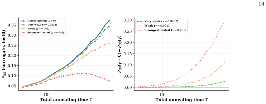
assumptions (7)
- standard math Suzuki–Trotter mapping gives an equivalent classical worldline model for the transverse-field Ising Hamiltonian.
- domain assumption The worldline magnetization susceptibility χm obeys fluctuation–dissipation and scales as 1/Δ(s)^2 near criticality.
- domain assumption The peak of χm correctly locates the critical/min-gap region for schedule construction.
- domain assumption The Roland–Cerf condition Eq. (4) is the appropriate benchmark for finite-time optimality.
- ad hoc to paper The exact Roland–Cerf time allocation is captured by F(s)=∫Δ^{-2}/∫Δ^{-2}, i.e. the transition matrix element in Eq. (4) is constant or negligible.
- ad hoc to paper Oscillatory PGS(T) under the Roland–Cerf schedule is caused by multilevel coherent interference.
- domain assumption Lindblad single-qubit dephasing at rates γ∈{0.001,...,0.05} is representative for robustness conclusions.
Cite this review
Pith. "Pith review of Worldline-Susceptibility Scheduling for Quantum Annealing Beyond Local-Adiabatic Evolution." pith.science (2026). https://pith.science/paper/AWWBX4V7
@misc{pith2026260714282,
  author       = {Pith},
  title        = {Pith review of: Worldline-Susceptibility Scheduling for Quantum Annealing Beyond Local-Adiabatic Evolution},
  year         = {2026},
  howpublished = {\url{https://pith.science/paper/AWWBX4V7}},
  note         = {Machine review of arXiv:2607.14282}
}
read the original abstract
The performance of quantum annealing depends critically on how the available annealing time is distributed along the evolution. Although the Roland Cerf local adiabatic schedule is theoretically optimal, it requires complete knowledge of the instantaneous spectral gap, making it impractical for large optimization problems. We propose a computationally inexpensive surrogate schedule based on the worldline magnetization susceptibility measured during simulated quantum annealing. The susceptibility is obtained directly from equilibrium Monte Carlo sampling and identifies the critical region of the anneal without requiring spectral information. Using exact diagonalization of Sherrington Kirkpatrick spin glass instances as ground truth, we show that the resulting schedule consistently outperforms conventional linear annealing and, for a substantial fraction of instances, also surpasses the exact Roland Cerf schedule. We demonstrate that this unexpected behaviour originates from two finite time failure modes of exact local adiabatic scheduling a boundary gap trap, in which the minimum spectral gap occurs at the end of the anneal, and an oscillatory instability caused by excessively localized time allocation around an interior minimum gap. These results suggest that robust scheduling based on inexpensive equilibrium observables can outperform exact spectral gap based strategies under realistic finite time conditions. The complete methodology is implemented in the open source Qanneal framework.
Figures


Figures from the paper (11 more)




Reference graph
Works this paper leans on
-
[1]
In such instances, the Roland–Cerf prescription faithfully allocates the majority of the available runtime to the region where the gap is smallest
Boundary-Gap Trap The first finite-time failure mode occurs when the mini- mum spectral gap is located at, or extremely close to, the end of the annealing trajectory. In such instances, the Roland–Cerf prescription faithfully allocates the majority of the available runtime to the region where the gap is smallest. While this allocation is formally consiste...
-
[2]
Here the minimum 10 spectral gap is located well inside the annealing interval rather than at its endpoint
Oscillatory Instability The second finite-time failure mode is qualitatively dif- ferent from the boundary-gap trap. Here the minimum 10 spectral gap is located well inside the annealing interval rather than at its endpoint. One would therefore expect the Roland–Cerf schedule to provide an excellent approx- imation to the optimal adiabatic evolution. Surp...
-
[3]
Kadowaki and H
T. Kadowaki and H. Nishimori, Physical Review E58, 5355 (1998)
1998
- [4]
-
[5]
G. E. Santoro, R. Martˇ on´ ak, E. Tosatti, and R. Car, Science295, 2427 (2002)
2002
-
[6]
Lucas, Frontiers in Physics2, 5 (2014)
A. Lucas, Frontiers in Physics2, 5 (2014)
2014
-
[7]
Albash and D
T. Albash and D. A. Lidar, Reviews of Modern Physics 90, 015002 (2018)
2018
-
[8]
Crosson and D
E. Crosson and D. A. Lidar, Nature Reviews Physics3, 466 (2020)
2020
Show all 60 references
-
[9]
A. King, J. Raymond, T. Lanting, R. Harris, A. Zucca, F. Altomare, A. Berkley, K. Boothby, S. Ejtemaee, C. En- derud, E. Hoskinson, S. Huang, E. Ladizinsky, A. MacDon- ald, G. Marsden, R. Molavi, T. Oh, G. Poulin-Lamarre, M. Reis, C. Rich, Y. Sato, N. Tsai, M. Volkmann, J. Whi...
2022
-
[10]
Hauke, H
P. Hauke, H. Katzgraber, W. Lechner, H. Nishimori, and W. Oliver, Reports on Progress in Physics83(2019)
2019
-
[11]
Laumann, C
C. Laumann, C. Laumann, R. Moessner, A. Scardicchio, and S. Sondhi, The European Physical Journal Special Topics224, 75 (2014)
2014
-
[12]
Roland and N
J. Roland and N. J. Cerf, Physical Review A65, 042308 (2002)
2002
-
[13]
Jansen, M.-B
S. Jansen, M.-B. Ruskai, and R. Seiler, Journal of Mathe- matical Physics48, 102111 (2007)
2007
-
[14]
D. A. Lidar, A. Rezakhani, and A. Hamma, Adiabatic approximation with exponential accuracy for many-body systems and quantum computation (2008)
2008
-
[15]
Suzuki, Progress of Theoretical Physics56, 1454 (1976)
M. Suzuki, Progress of Theoretical Physics56, 1454 (1976)
1976
-
[16]
H. F. Trotter, Proceedings of the American Mathematical Society10, 545 (1959)
1959
-
[17]
Bando and H
Y. Bando and H. Nishimori, Simulated quantum anneal- ing as a simulator of nonequilibrium quantum dynamics (2021)
2021
-
[18]
Mbeng, L
G. Mbeng, L. Privitera, L. Arceci, and G. Santoro, Dy- namics of simulated quantum annealing in random Ising chains (2018)
2018
-
[19]
You, Y.-W
W. You, Y.-W. Li, and S. Gu, Physical review. E, Sta- tistical, nonlinear, and soft matter physics76 2 Pt 1, 022101 (2007)
2007
-
[20]
A. F. Albuquerque, F. Alet, C. Sire, and S. Capponi, Quantum critical scaling of fidelity susceptibility (2009)
2009
-
[21]
Pelofske, Mapping state transition susceptibility in quantum annealing (2022)
E. Pelofske, Mapping state transition susceptibility in quantum annealing (2022)
2022
-
[22]
Ovits and L
E. Ovits and L. Wolf, International Conference on Learn- ing Representations (2021)
2021
-
[23]
Sherrington and S
D. Sherrington and S. Kirkpatrick, Physical Review Let- ters35, 1792 (1975)
1975
-
[24]
Rieger and A
H. Rieger and A. Young, Physical review letters72 26, 4141 (1994)
1994
-
[25]
A. Kiss, G. Zar´ and, and I. Lovas, Physical Review B (2023)
2023
-
[26]
Y. W. Koh, Effects of low-lying excitations on ground- state energy and energy gap of the Sherrington- Kirkpatrick model in a transverse field (2016)
2016
-
[27]
Cullimore, M
M. Cullimore, M. Everitt, M. Ormerod, J. Samson, R. Wil- son, and A. Zagoskin, Relationship between minimum gap and success probability in adiabatic quantum computing (2011)
2011
-
[28]
Rakcheev and A
A. Rakcheev and A. L¨ auchli, Physical Review A (2022)
2022
-
[29]
L. P. Garc ´ ıa-Pintos, L. Brady, J. Bringewatt, and Y.-K. Liu, Physical review letters130 14, 140601 (2022)
2022
-
[30]
Muthukrishnan, T
S. Muthukrishnan, T. Albash, and D. A. Lidar, Tunneling and speedup in quantum optimization for permutation- symmetric problems (2015)
2015
-
[31]
J¨ org, F
T. J¨ org, F. Krzakala, F. Krzakala, J. Kurchan, A. C. Maggs, and J. Pujos, Energy gaps in quantum first-order mean-field–like transitions: The problems that quantum annealing cannot solve (2009)
2009
-
[32]
Young, S
A. Young, S. Knysh, and V. Smelyanskiy, Physical review letters104 2, 020502 (2009)
2009
-
[33]
S. N. Shevchenko, S. Ashhab, and F. Nori, Physics Reports 492, 1 (2010)
2010
-
[34]
J. R. Finˇ zgar, M. Schuetz, J. K. Brubaker, H. Nishimori, and H. Katzgraber, Physical Review Research (2023)
2023
-
[35]
Morita and H
S. Morita and H. Nishimori, Convergence of Quantum An- nealing with Real-Time Schrodinger Dynamics(General) (2007)
2007
-
[36]
B. Heim, T. F. Rønnow, S. Isakov, and M. Troyer, Science 348, 215 (2014)
2014
-
[37]
A. King, S. Suzuki, J. Raymond, A. Zucca, T. Lant- ing, F. Altomare, A. Berkley, S. Ejtemaee, E. Hoskinson, S. Huang, E. Ladizinsky, A. MacDonald, G. Marsden, T. Oh, G. Poulin-Lamarre, M. Reis, C. Rich, Y. Sato, J. Whittaker, J. J. Yao, R. Harris, D. A. Lidar, H. Nishi- mori, ...
2022
-
[38]
Willsch, M
D. Willsch, M. Willsch, F. Jin, K. Michielsen, and H. Raedt, Comput. Phys. Commun.278, 108411 (2021)
2021
-
[39]
Singh, L
S. Singh, L. Nagpal, V. Chauhan, and S. R. Hassan, Qan- neal: A C++17/Python framework for simulated quan- 14 tum annealing — user manual (2026), software manual accompanying theqannealv2.0.0 release
2026
-
[40]
R. H. Swendsen and J.-S. Wang, Physical Review Letters 58, 86 (1987)
1987
-
[41]
Marshall, D
J. Marshall, D. Venturelli, I. Hen, and E. Rieffel, Power of Pausing: Advancing Understanding of Thermalization in Experimental Quantum Annealers (2018)
2018
-
[42]
Albash and J
T. Albash and J. Marshall, Comparing Relaxation Mech- anisms in Quantum and Classical Transverse-Field An- nealing (2020)
2020
-
[43]
Martˇ on´ ak, G
R. Martˇ on´ ak, G. E. Santoro, and E. Tosatti, Physical Review B66, 094203 (2002). 15 Appendix A: Qanneal: An Open-Source F ramework for Simulated Quantum Annealing All simulated-quantum-annealing results in this work were produced with qanneal, an open-source, research-grade...
2002
-
[44]
import qanneal; print(qanneal.__version__)
Installation qanneal requires Python ≥ 3.11, NumPy, and a C++17 compiler (GCC ≥ 9, Clang ≥ 10, or MSVC 2019+); OpenMP is optional but recommended for replica/slice parallelism, and dimod/networkx are optional for BQM/- graph problem inputs. From the repository root: python -m ...
2019
-
[45]
(1)–(2) of the main text are accepted directly; the package auto-detects dense arrays, sparse edge lists, dictionaries, dimod binary quadratic models, and networkx graphs
Problem setup Both the Ising and QUBO conventions of Eqs. (1)–(2) of the main text are accepted directly; the package auto-detects dense arrays, sparse edge lists, dictionaries, dimod binary quadratic models, and networkx graphs. A Sherrington–Kirkpatrick instance, as used thr...
-
[46]
Suzuki–T rotter representation qanneal samples the equilibrium density matrix of the transverse-field Ising Hamiltonian, Eq. (1) of the main text, by Trotterizing the imaginary-time partition func- tion into M classical replicas (“slices”) coupled along imaginary time with str...
-
[47]
sa" Classical simulated annealing (Metropolis)
Engines available Engine (method=) What it simulates "sa" Classical simulated annealing (Metropolis) "sqa"Discrete-time Suzuki–Trotter SQA "sqapt" SQA + replica exchange, ( β, Γ) lad- der "ctpimc" Continuous-time path-integral Monte Carlo [41] "sqa chi" SQA with the worldline-...
-
[48]
II.C of the main text is implemented directly as the SQAChiAnnealer class
The worldline-susceptibility schedule (sqa chi) The surrogate schedule constructed in Sec. II.C of the main text is implemented directly as the SQAChiAnnealer class. Its execution mirrors the workflow of Sec. II.D one- to-one:
-
[49]
χm(s) [Eq
Pilot scan. χm(s) [Eq. (8) of the main text] is measured at scan points values of the annealing parameter s∈ [0, 1], each from an independently randomized worldline (not carried over between grid points, so every estimate is statistically inde- pendent), using scan burn burn-i...
-
[50]
Time allocation.The pilot profile is floor- regularized, w(s) = max χm(s),chi floor fraction·max s′ χm(s′) , (A3) and inverted via the cumulative map of Eqs. (12)– (14) of the main text to place num steps sched- ule points at equal increments of accumulated sus- ceptibility we...
-
[51]
Production anneal.A short thermal ramp (fraction beta ramp fraction of the step budget, default 0.3) equilibrates the worldlines at the target inverse temperature at fixed γstart; the γ(s) trajectory from step 2 is then executed on a fresh worldline through the same checkerboa...
-
[52]
III.G (Figs
Reproducing the results of this paper The parameter grid of Sec. III.G (Figs. 14–15) is repro- duced by loopingrun chiover M∈ {8,16,32,64},(A4) β∈ {2,5,10,20},(A5) with scan points=16, scan sweeps=30, scan burn=10, replicas=4, and comparing the resulting s star against the exa...
-
[53]
Parameter grid used for the SQA-parameter robustness study (Sec
Parameters used in this work Parameter Values Trotter slicesM{8,16,32,64} Inverse temperatureβ{2,5,10,20} Pilot scan points 16 Pilot scan sweeps / burn-in 30 / 10 Replicas 4 Regularization floor 10 −6 ×max s χm Thermal ramp fraction 0.3 TABLE IV. Parameter grid used for the SQ...
-
[54]
Availability qanneal is released under the Apache License 2.0. Source code, build instructions, and the complete manual from which this appendix is condensed are available at https://pypi.org/project/qanneal/ Users of the package for scheduling or SQA simulation are asked to c...
-
[55]
III C.B was diagnosed entirely from unitary, closed-system propaga- tion
Open-system control: does decoherence erase the oscillatory instability? The oscillatory instability identified in Sec. III C.B was diagnosed entirely from unitary, closed-system propaga- tion. Because coherent multilevel interference is precisely the kind of effect that depha...
-
[56]
Does the surrogate schedule’s advantage survive the same dephasing? Having established that decoherence does not erase the Roland–Cerf oscillation, we next ask whether the worldline-susceptibility schedule’s performance is similarly robust, since the original submission tested...
-
[57]
Is the residuals ∗ ED–s∗ SQ disagreement a T rotter discretization bias? Section III.A reports a residual offset between the exact- diagonalization crossing point s∗ ED and the worldline- susceptibility crossing point s∗ SQ. Since s∗ SQ is extracted from a Suzuki–Trotter-discr...
-
[58]
Held-out validation of the∆ ∗ failure threshold Section III.D reports that Roland–Cerf failure (boundary- gap or oscillatory) becomes more likely as the minimum spectral gap ∆ ∗ shrinks, with an indicative threshold estimated from six curated instances without a held-out test....
-
[59]
To determine whether the oscillatory and boundary-gap mechanisms of Sec
Do the Roland–Cerf failure rates persist at larger system sizes? Section III.D shows that the fraction of instances exhibit- ing the boundary-gap trap increases with n over the six system sizes studied, but does not report confidence inter- vals on the underlying class rates. ...
-
[60]
Summary The five checks above address the main quantitative and methodological gaps left open by the original submission: they confirm that the oscillatory instability of Sec. III C.B is a genuine coherent effect that survives moderate dephas- ing rather than a numerical artif...
Reviewed August 2, 2026 · model on record in the stance chip above.
Discussion (0). Continue with ORCID to comment.