REVIEW 2 major objections 6 minor 139 references
Resistive GRMHD simulations of neutron-star mergers show the electric field parallel to the magnetic field can reach 10% of the total field in low-density disks, an effect ideal MHD sets to zero.
Reviewed by Pith at T0; open to challenge. T0 means a machine referee read the full paper against a public rubric. the ladder, T0–T4 →
T0 review · grok-4.5
2026-07-14 03:58 UTC pith:B3D4NC3D
load-bearing objection Solid BAM infrastructure paper with careful tests; the 10% parallel-E number is real under their setup but rests on a density-only conductivity that zeros outside the star. the 2 major comments →
Extending the infrastructure of the BAM code towards resistive general-relativistic magnetohydrodynamics: tests and first applications
The pith
A machine-rendered reading of the paper's core claim, the machinery that carries it, and where it could break.
Core claim
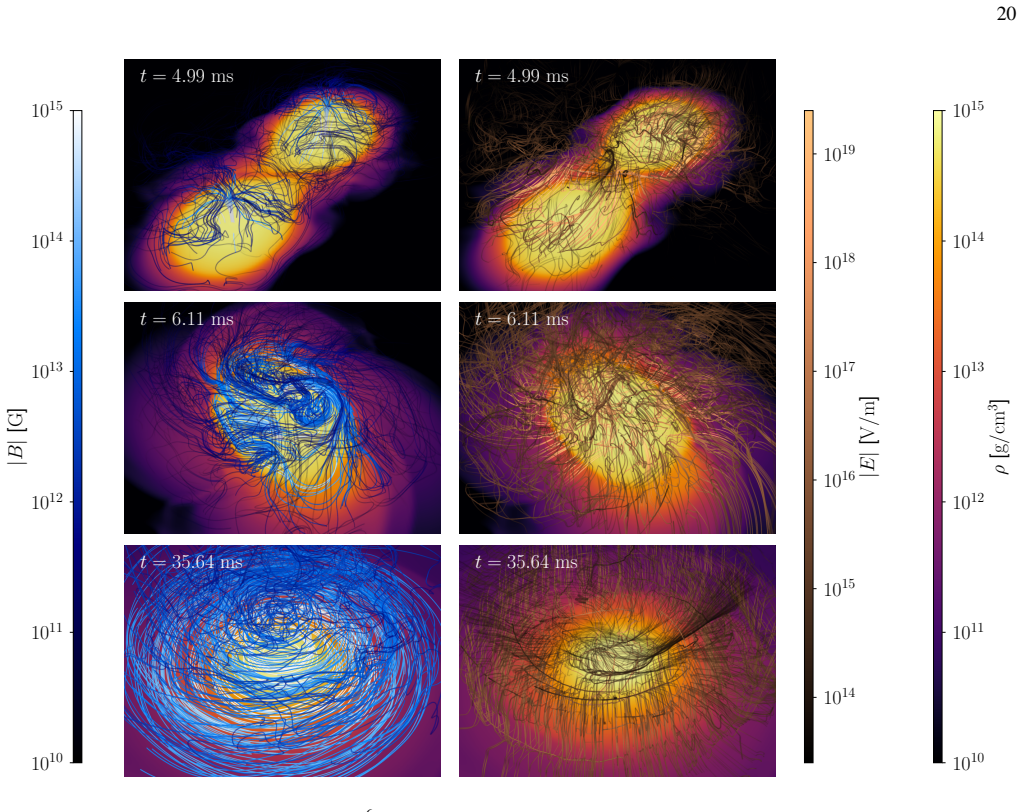
In binary-neutron-star mergers evolved with resistive GRMHD, the electric-field component parallel to the magnetic field reaches values up to about 10 percent of the total electric-field strength in the low-density disk around the remnant, while remaining negligible inside the dense stellar cores; this component is identically zero under the ideal-MHD approximation.
What carries the argument
A resistive GRMHD module that evolves the electric field with an implicit-explicit Runge-Kutta integrator, an isotropic scalar Ohm's law, hyperbolic divergence cleaning, and a density-tracking conductivity profile that interpolates between highly conductive stellar interiors and a vacuum exterior.
Load-bearing premise
Electrical conductivity is prescribed by a simple density-tracking isotropic scalar that is zero outside the star and constant inside; realistic temperature- and composition-dependent conductivities are not yet used.
What would settle it
Higher-resolution resistive BNS simulations that employ temperature- and composition-dependent conductivities and measure whether the parallel electric-field fraction in the post-merger disk still reaches order 10 percent, or drops to levels consistent with pure numerical noise.
If this is right
- Long-term post-merger remnant evolution and jet-launching calculations must retain finite conductivity at least in low-density regions.
- Magnetic reconnection and Ohmic dissipation become accessible mechanisms for energy release and electromagnetic flares once the ideal-MHD constraint is dropped.
- Mass-ejection diagnostics and magnetic-field amplification rates acquire a measurable dependence on conductivity that ideal-MHD runs cannot capture.
- The same infrastructure can later incorporate anisotropic or force-free exterior currents without rewriting the evolution scheme.
Where Pith is reading between the lines
- If the 10 percent parallel electric field survives more realistic microphysics, polar-jet models that currently assume ideal MHD may systematically mis-estimate Poynting flux and reconnection rates.
- The same resistive framework offers a controlled route to test whether mean-field dynamo or Hall terms alter the large-scale field topology that ideal MHD currently produces.
- A clean observational discriminator would be a late-time electromagnetic signature whose spectrum or polarization depends on residual resistivity in the disk.
Editorial analysis
A structured set of objections, weighed in public.
Referee Report
Summary. The manuscript extends the BAM numerical-relativity code from ideal to resistive GRMHD by evolving the electric field with an IMEX Runge–Kutta scheme, hyperbolic divergence cleaning, and an isotropic scalar Ohm’s law. After an extensive suite of special-relativistic benchmarks (shock tubes, monopole cleaning, Alfvén wave, current sheet, blast waves, charged vortex, rotor, KHI) and isolated magnetized TOV stars, the authors present short BNS evolutions at several conductivities and compare them to BAM’s ideal module. The main application result is that the electric-field component parallel to B, identically zero in ideal GRMHD, can reach up to ~10% of |E| in low-density post-merger regions under their density-tracking conductivity profile.
Significance. Resistive GRMHD BNS simulations remain scarce; a validated resistive module in a widely used NR code is a genuine community contribution. The test suite is thorough, with direct comparisons to analytic solutions and to BAM’s independent ideal implementation, and the IMEX/primitive-recovery infrastructure is described carefully enough to be useful. The first BNS applications are preliminary (piecewise-polytropic EOS, modest resolution, simplified σ) but already indicate where non-ideal effects may matter. Strengths include explicit convergence checks (current sheet, charged vortex), multi-resolution BNS runs, and honest discussion of atmosphere and exterior treatments. If the caveats on conductivity modeling are stated clearly, the paper is a solid methods-plus-first-applications contribution.
major comments (2)
- Abstract and §V C (Figs. 26–27): the headline claim that E∥/|E| reaches ~10% in the post-merger disk is measured with the density-tracking profile of Eq. (73), which forces σ→0 below D_thr and yields an electrovacuum exterior. The paper itself notes (§IV J) that a force-free exterior is more realistic and that the present choice is for simplicity. In vacuum Maxwell evolution a nonzero parallel component is not surprising; the 10% figure therefore cannot yet be read as a robust statement about non-ideal plasma physics inside a conducting disk. Please either (i) rephrase the abstract/conclusion to state that the result is under this specific σ model and electrovacuum exterior, or (ii) add a controlled comparison (even 2D or short 3D) with a phenomenological force-free current of the type already sketched in the code, so the reader can judge how much of the signal survives a more physical e
- §V D and Fig. 28: ejecta masses for the ideal module and the σ0=10^6 resistive runs differ by ~50–100% (HM case >100%), which the text attributes to “implementation differences” (conservative-to-primitive, timestepping, EM–spacetime coupling, lapse). That systematic is larger than the reported physical trend with conductivity in the LM series. Before using ideal-vs-resistive ejecta differences to support physical conclusions, quantify the ideal–resistive discrepancy more carefully (e.g., identical reconstruction/Riemann settings where possible, or a controlled σ→∞ limit study) and assign a clearer numerical uncertainty so the conductivity trend is not overstated.
minor comments (6)
- §II D / footnote 1: the conversion factor between code conductivity and cgs units is given once; a short table or explicit statement of what σ0=10^2, 10^4, 10^6 correspond to in s^−1 (and relative to expected crust/core values) would help non-specialists place the runs.
- §III C: the choice of light-speed characteristic speeds for the LLF solver is justified, but the text should briefly note how this affects the ideal-limit comparison in the BNS runs (extra numerical diffusion relative to the ideal module’s eigenstructure).
- Figs. 26–27: isodensity contours are helpful; adding a panel or inset of σ (or D) on the same slices would make the connection between low conductivity and high E∥ immediate.
- §IV J / Fig. 21: the Ohmic-diffusion timescale argument is clear for σ0=10^2 vs 2×10^2; a one-line estimate of λ_B used would make the comparison fully quantitative.
- Table I naming (LMσ2_R1 etc.) is dense; a short legend in the caption mapping superscripts to σ0 values would improve readability.
- Minor typography: “bamcode”/“bam” capitalization is inconsistent in the title and body; “Heaviside–Lorentz” and unit conventions are fine but could be stated once in a dedicated paragraph for reproducibility.
Circularity Check
No circularity: the 10% parallel-E result is a direct numerical measurement under a free conductivity ansatz, not a tautology or fitted prediction.
full rationale
The paper implements a standard resistive GRMHD system (Maxwell + isotropic Ohm’s law + IMEX time integration) following external literature (Palenzuela et al., Dionysopoulou et al., Izquierdo et al.). Validation consists of external analytic benchmarks (shock tube, Alfvén wave, self-similar current sheet, charged vortex, etc.) and side-by-side comparison with BAM’s independent ideal-GRMHD module. The conductivity profile (Eq. 73) is an explicit free-parameter ansatz (density-tracking, zero in the atmosphere) chosen for numerical exploration, not fitted to any target observable. The strongest claim—E∥/|E| reaching ~10% in the low-density post-merger disk—is simply the measured value of Eq. (75) on the evolved fields; it is identically zero only in the ideal limit by construction of Ohm’s law, so the non-zero result is a genuine output of the resistive evolution, not a re-labeling of an input. No uniqueness theorem, self-citation chain, or fitted parameter is load-bearing for the claim. Minor self-citations (e.g., to the authors’ prior ideal-GRMHD paper) supply only the base infrastructure and are independently cross-checked. The derivation chain is therefore self-contained against external tests; any limitations are physical (simplified EOS, electrovacuum exterior) rather than circular.
Axiom & Free-Parameter Ledger
free parameters (4)
- σ₀ (maximum conductivity) =
10²–10⁶
- atmosphere fraction f_atm and threshold f_thr =
f_atm=10^{-11}, f_thr=1.1
- divergence-cleaning rates κ_ϕ = κ_ψ =
1
- initial magnetic-field strength A_b =
1000 (BNS)
axioms (4)
- domain assumption Isotropic scalar Ohm’s law J^i = q v^i + W σ [E^i + ε^{ijk} v_j B_k − (v·E) v^i]
- domain assumption Piecewise-polytropic fit to SLy EOS plus thermal Γ_th=1.75
- ad hoc to paper Density-tracking conductivity profile σ = σ₀ max(1 − D_thr/D, 0)²
- standard math 3+1 Einstein equations in Z4c formulation with 1+log and Γ-driver
read the original abstract
Many astrophysical phenomena, including pulsars and short gamma-ray bursts, are associated with the extremely strong magnetic fields present in neutron stars and neutron star mergers. While the ideal magnetohydrodynamic approximation, which assumes infinite conductivity, provides an excellent description of the neutron-star interior, it cannot capture non-ideal processes such as Ohmic dissipation and magnetic reconnection. To overcome this limitation, we present an extension of the numerical-relativity code BAM incorporating a resistive general-relativistic magnetohydrodynamic (GRMHD) description. We validate the new implementation through an extensive suite of special-relativistic magnetohydrodynamic benchmark tests and by performing stable simulations of isolated and binary neutron star systems. For the latter, we investigate the impact of finite conductivity on magnetic-field amplification, mass ejection, and non-ideal GRMHD effects. In particular, we find that the component of the electric field parallel to the magnetic field, which is zero in the ideal case, can reach up to 10% of the total electric field strength. This highlights the potential importance of non-ideal effects for accurately modeling the long-term evolution of post-merger remnants, particularly in low-density regions. Although the present study is restricted to simplified piecewise-polytropic equations of state, it demonstrates the capabilities of the new resistive GRMHD framework and paves the way for future investigations employing more realistic microphysics.
Figures









Reference graph
Works this paper leans on
-
[1]
B. P. Abbottet al.(LIGO Scientific, Virgo), Phys. Rev. Lett. 119, 161101 (2017), arXiv:1710.05832 [gr-qc]
Pith/arXiv arXiv 2017
-
[2]
850, L39 (2017), arXiv:1710.05836 [astro-ph.HE]
B.P.Abbottet al.(LIGOScientific,Virgo),Astrophys.J.Lett. 850, L39 (2017), arXiv:1710.05836 [astro-ph.HE]
Pith/arXiv arXiv 2017
-
[3]
Arcaviet al., Nature551, 64 (2017), arXiv:1710.05843 [astro-ph.HE]
I. Arcaviet al., Nature551, 64 (2017), arXiv:1710.05843 [astro-ph.HE]
Pith/arXiv arXiv 2017
-
[4]
ej [" ] 103 LMid R1 LMf2 R1 LMf4 R1 LMf6 R1 00 25 50
D.Kasen,B.Metzger,J.Barnes,E.Quataert,andE.Ramirez- Ruiz,Nature551,80(2017),arXiv:1710.05463[astro-ph.HE]. 24 FIG. 27. Relative electric field parallel to the magnetic field for the HM simulations with𝜎0 ={10 2,10 4,10 6}at the R1 resolution. Each row shows snapshots for one simulation in the𝑥𝑦-plane, while each column represents different times in the si...
Pith/arXiv arXiv 2017
-
[5]
A. Goldsteinet al., Astrophys. J. Lett.848, L14 (2017), arXiv:1710.05446 [astro-ph.HE]
Pith/arXiv arXiv 2017
-
[6]
V. Savchenkoet al., Astrophys. J. Lett.848, L15 (2017), arXiv:1710.05449 [astro-ph.HE]
Pith/arXiv arXiv 2017
-
[7]
Brandenburg and K
A. Brandenburg and K. Subramanian, Physics Reports417, 1 (2005)
2005
-
[8]
M. Ruiz, R. N. Lang, V. Paschalidis, and S. L. Shapiro, Astro- phys.J.Lett.824,L6(2016),arXiv:1604.02455[astro-ph.HE]
Pith/arXiv arXiv 2016
-
[9]
P. Mösta, D. Radice, R. Haas, E. Schnetter, and S. Bernuzzi, Astrophys. J. Lett.901, L37 (2020), arXiv:2003.06043 [astro- ph.HE]
Pith/arXiv arXiv 2020
-
[10]
K.Kiuchi,A.Reboul-Salze,M.Shibata,andY.Sekiguchi,Nat Astron8, 298 (2024)
2024
-
[11]
D.R.Lorimer,LivingRev.Rel.11,8(2008),arXiv:0811.0762 [astro-ph]
Pith/arXiv arXiv 2008
-
[12]
T. M. Tauriset al., Astrophys. J.846, 170 (2017), arXiv:1706.09438 [astro-ph.HE]
Pith/arXiv arXiv 2017
-
[13]
D. J. Price and S. Rosswog, Science312, 719 (2006)
2006
-
[14]
Kiuchi, P
K. Kiuchi, P. Cerdá-Durán, K. Kyutoku, Y. Sekiguchi, and M. Shibata, Phys. Rev. D92, 124034 (2015)
2015
-
[15]
Giacomazzo, J
B. Giacomazzo, J. Zrake, P. C. Duffell, A. I. MacFadyen, and R. Perna, ApJ809, 39 (2015)
2015
-
[16]
R. Aguilera-Miret, J.-E. Christian, S. Rosswog, and C. Palen- zuela, Mon. Not. Roy. Astron. Soc.542, 3067 (2025), arXiv:2504.10604 [astro-ph.HE]
arXiv 2025
-
[17]
E. M. Gutiérrez, D. Radice, J. Fields, and J. M. Stone, arXiv e-prints , arXiv:2601.20953 (2026), arXiv:2601.20953 [astro- ph.HE]. 25
arXiv 2026
-
[18]
M. D. Duez, Y. T. Liu, S. L. Shapiro, M. Shibata, and B. C. Stephens, Physical Review Letters96, 031101 (2006)
2006
-
[19]
D87, 121302 (2013)
D.M.Siegel,R.Ciolfi,A.I.Harte,andL.Rezzolla,Phys.Rev. D87, 121302 (2013)
2013
-
[20]
R.Aguilera-Miret, C.Palenzuela, F.Carrasco,andD.Viganò, Phys. Rev. D108, 103001 (2023), arXiv:2307.04837 [astro- ph.HE]
Pith/arXiv arXiv 2023
-
[21]
E. R. Most, Phys. Rev. D108, 123012 (2023), arXiv:2311.03333 [astro-ph.HE]
Pith/arXiv arXiv 2023
-
[22]
A. Reboul-Salze, P. Barrère, K. Kiuchi, J. Guilet, R.Raynaud, S. Fujibayashi, and M. Shibata, Astron. Astrophys.699, A4 (2025), arXiv:2411.19328 [astro-ph.HE]
arXiv 2025
-
[23]
R. D. Blandford and R. L. Znajek, Monthly Notices of the Royal Astronomical Society179, 433 (1977)
1977
-
[24]
Rezzolla, B
L. Rezzolla, B. Giacomazzo, L. Baiotti, J. Granot, C. Kou- veliotou, and M. A. Aloy, The Astrophysical Journal732, L6 (2011)
2011
-
[25]
K.Kiuchi,K.Kyutoku,Y.Sekiguchi,M.Shibata,andT.Wada, Physical Review D90, 041502 (2014)
2014
-
[26]
Palenzuela, S
C. Palenzuela, S. L. Liebling, D. Neilsen, L. Lehner, O. L. Caballero,E.O’Connor,andM.Anderson,PhysicalReviewD 92, 044045 (2015)
2015
-
[27]
Kiuchi, K
K. Kiuchi, K. Kyutoku, Y. Sekiguchi, and M. Shibata, Phys. Rev. D97, 124039 (2018)
2018
-
[28]
W. Cook, B. Daszuta, J. Fields, P. Hammond, S. Albanesi, F. Zappa, S. Bernuzzi, and D. Radice, Astrophys. J. Suppl. 277, 3 (2025), arXiv:2311.04989 [gr-qc]
Pith/arXiv arXiv 2025
-
[29]
E. M. Gutiérrez, W. Cook, D. Radice, S. Bernuzzi, J. Fields, P. Hammond, B. Daszuta, H. Bandyopadhyay, and M. Jacobi, arXiv e-prints , arXiv:2506.18995 (2025), arXiv:2506.18995 [astro-ph.HE]
arXiv 2025
-
[30]
Chabanov, S
M. Chabanov, S. D. Tootle, E. R. Most, and L. Rezzolla, The Astrophysical Journal945, L14 (2023)
2023
-
[31]
Schianchi, P
A.Neuweiler,T.Dietrich,B.Brügmann,E.Giangrandi,K.Ki- uchi, F. Schianchi, P. Mösta, S. Shankar, B. Giacomazzo, and M. Shibata, Physical Review D110, 084046 (2024)
2024
-
[32]
C. Musolino, L. Rezzolla, and E. R. Most, Astrophys. J. Lett. 984, L61 (2025), arXiv:2410.06253 [astro-ph.HE]
Pith/arXiv arXiv 2025
-
[33]
Kiuchi, inNew Frontiers in GRMHD Simulations, edited by C
K. Kiuchi, inNew Frontiers in GRMHD Simulations, edited by C. Bambi, Y. Mizuno, S. Shashank, and F. Yuan (Springer Nature, Singapore, 2025) pp. 529–572
2025
-
[34]
A. Schmitt and P. Shternin, Astrophys. Space Sci. Libr.457, 455 (2018), arXiv:1711.06520 [astro-ph.HE]
Pith/arXiv arXiv 2018
-
[35]
Harutyunyan and A
A. Harutyunyan and A. Sedrakian, Physical Review C94, 025805 (2016)
2016
-
[36]
Harutyunyan, A
A. Harutyunyan, A. Sedrakian, N. T. Gevorgyan, and M. V. Hayrapetyan, Physical Review C109, 055804 (2024)
2024
-
[37]
Harutyunyan, A
A. Harutyunyan, A. Nathanail, L. Rezzolla, and A. Sedrakian, European Physical Journal A54, 191 (2018)
2018
-
[38]
Dionysopoulou, D
K. Dionysopoulou, D. Alic, C. Palenzuela, L. Rezzolla, and B. Giacomazzo, Physical Review D88, 044020 (2013)
2013
-
[39]
Palenzuela, Monthly Notices of the Royal Astronomical Society431, 1853 (2013)
C. Palenzuela, Monthly Notices of the Royal Astronomical Society431, 1853 (2013)
2013
-
[40]
P. C.-K. Cheong, D. Y. T. Pong, A. K. L. Yip, and T. G. F. Li, The Astrophysical Journal Supplement Series261, 22 (2022)
2022
-
[41]
Franceschetti and R
K. Franceschetti and R. De Pietri, Physical Review D111, 124033 (2025)
2025
- [42]
-
[43]
Palenzuela, L
C. Palenzuela, L. Lehner, M. Ponce, S. L. Liebling, M. An- derson, D. Neilsen, and P. Motl, Physical Review Letters111, 061105 (2013)
2013
-
[44]
Neilsen, and P
C.Palenzuela,L.Lehner,S.L.Liebling,M.Ponce,M.Ander- son, D. Neilsen, and P. Motl, Physical Review D88, 043011 (2013)
2013
-
[45]
Ponce, C
M. Ponce, C. Palenzuela, L. Lehner, and S. L. Liebling, Phys. Rev. D90, 044007 (2014)
2014
-
[46]
Dionysopoulou, D
K. Dionysopoulou, D. Alic, and L. Rezzolla, Physical Review D92, 084064 (2015)
2015
-
[47]
Brügmann, J
B. Brügmann, J. A. González, M. Hannam, S. Husa, U. Sper- hake, and W. Tichy, Physical Review D77, 024027 (2008)
2008
-
[48]
Thierfelder, S
M. Thierfelder, S. Bernuzzi, and B. Brügmann, Physical Re- view D84, 044012 (2011)
2011
-
[49]
Palenzuela, L
C. Palenzuela, L. Lehner, O. Reula, and L. Rezzolla, Monthly Notices of the Royal Astronomical Society394, 1727 (2009)
2009
-
[50]
R. Mbarek, J. Wu, and E. R. Most, arXiv e-prints , arXiv:2605.24083 (2026), arXiv:2605.24083 [astro-ph.HE]
Pith/arXiv arXiv 2026
-
[51]
Bernuzzi and D
S. Bernuzzi and D. Hilditch, Physical Review D81, 084003 (2010)
2010
-
[52]
Brügmann, Physical Review D88, 084057 (2013)
D.Hilditch,S.Bernuzzi,M.Thierfelder,Z.Cao,W.Tichy,and B. Brügmann, Physical Review D88, 084057 (2013)
2013
-
[53]
C.Bona,J.Stela,J.Massó,andE.Seidel,inProceedings of the Seventh Marcel Grossman Meeting on Recent Developments in Theoretical and Experimental General Relativity, Gravitation, and Relativistic Field Theories(1996) p. 410
1996
-
[54]
Alcubierre, B
M. Alcubierre, B. Brügmann, P. Diener, M. Koppitz, D. Poll- ney,E.Seidel,andR.Takahashi,PhysicalReviewD67,084023 (2003)
2003
-
[55]
C. R. Evans and J. F. Hawley, The Astrophysical Journal332, 659 (1988)
1988
-
[56]
Shankar, P
S. Shankar, P. Mösta, S. R. Brandt, R. Haas, E. Schnetter, and Y. de Graaf, Class. Quantum Grav.40, 205009 (2023)
2023
-
[57]
Kiuchi, L
K. Kiuchi, L. E. Held, Y. Sekiguchi, and M. Shibata, Phys. Rev. D106, 124041 (2022)
2022
-
[58]
Z. B. Etienne, Y. T. Liu, and S. L. Shapiro, Phys. Rev. D82, 084031 (2010)
2010
-
[59]
Cipolletta, J
F. Cipolletta, J. V. Kalinani, B. Giacomazzo, and R. Ciolfi, Class. Quantum Grav.37, 135010 (2020)
2020
-
[60]
Dedner, F
A. Dedner, F. Kemm, D. Kröner, C. D. Munz, T. Schnitzer, and M. Wesenberg, Journal of Computational Physics175, 645 (2002)
2002
-
[61]
S.L.Liebling,L.Lehner,D.Neilsen,andC.Palenzuela,Phys. Rev. D81, 124023 (2010)
2010
-
[62]
A. J. Penner, Mon. Not. Roy. Astron. Soc.414, 1467 (2011), arXiv:1011.2976 [astro-ph.HE]
Pith/arXiv arXiv 2011
-
[63]
Mösta, B
P. Mösta, B. C. Mundim, J. A. Faber, R. Haas, S. C. Noble, T. Bode, F. Löffler, C. D. Ott, C. Reisswig, and E. Schnetter, Classical and Quantum Gravity31, 015005 (2014)
2014
-
[64]
N. Deppeet al., Phys. Rev. D105, 123031 (2022), arXiv:2109.12033 [gr-qc]
Pith/arXiv arXiv 2022
-
[65]
C. Palenzuela, B. Miñano, D. Viganò, A. Arbona, C. Bona- Casas, A. Rigo, M. Bezares, C. Bona, and J. Massó, Class. Quant. Grav.35, 185007 (2018), arXiv:1806.04182 [physics.comp-ph]
Pith/arXiv arXiv 2018
-
[66]
S. S. Komissarov, Monthly Notices of the Royal Astronomical Society382, 995 (2007)
2007
-
[67]
Tsamparlis,Special Relativity: An Introduction with 200 Problems and Solutions(Springer, Berlin, Heidelberg, 2010)
M. Tsamparlis,Special Relativity: An Introduction with 200 Problems and Solutions(Springer, Berlin, Heidelberg, 2010)
2010
-
[68]
A. Harutyunyan and A. Sedrakian, Phys. Rev. C94, 025805 (2016), arXiv:1605.07612 [astro-ph.HE]
Pith/arXiv arXiv 2016
-
[69]
J. A. Pons and D. Viganò, Living Rev Comput Astrophys5, 3 (2019)
2019
-
[70]
A. Harutyunyan, A. Sedrakian, N. T. Gevorgyan, and M. V. Hayrapetyan, Phys. Rev. C109, 055804 (2024), arXiv:2309.00893 [astro-ph.HE]. 26
arXiv 2024
-
[71]
T. Petrosyan, A.Harutyunyan, andA.Sedrakian,Phys.Rev.D 113, 063032 (2026), arXiv:2512.01044 [astro-ph.HE]
arXiv 2026
-
[72]
U.M.Ascher,S.J.Ruuth,andR.J.Spiteri,AppliedNumerical Mathematics25, 151 (1997)
1997
-
[73]
Pareschi and G
L. Pareschi and G. Russo, J Sci Comput25, 129 (2005)
2005
-
[74]
M. R. Izquierdo, L. Pareschi, B. Miñano, J. Massó, and C. Palenzuela, Class. Quantum Grav.40, 145014 (2023)
2023
-
[75]
Brügmann, Physical Review D54, 7361 (1996)
B. Brügmann, Physical Review D54, 7361 (1996)
1996
-
[76]
Brügmann, International Journal of Modern Physics D8, 85 (1999)
B. Brügmann, International Journal of Modern Physics D8, 85 (1999)
1999
-
[77]
T.Dietrich,S.Bernuzzi,M.Ujevic,andB.Brügmann,Physical Review D91, 124041 (2015)
2015
-
[78]
Bernuzzi and T
S. Bernuzzi and T. Dietrich, Physical Review D94, 064062 (2016)
2016
-
[79]
M. J. Berger and J. Oliger, Journal of Computational Physics 53, 484 (1984)
1984
-
[80]
M. J. Berger and P. Colella, Journal of Computational Physics 82, 64 (1989)
1989
discussion (0)
Sign in with ORCID, Apple, or X to comment. Anyone can read and Pith papers without signing in.