REVIEW 5 major objections 4 minor 40 references
Safe Deployment of Offline Reinforcement Learning via Input Convex Action Correction
T0 review · 5 major / 4 minor · reviewed 2026-08-06 · deepseek-v4-flash
Pith's one-line read A learned convex cost surface, descended by gradient at deployment, is what makes offline RL safe enough to control a polymerisation reactor.
desk verdict Worth a serious referee: the PICNN action-correction idea is interesting and the benchmark is useful, but the paper never states what cost the PICNN is trained to predict, which makes the core gradient update unverifiable as written. read the letter →
The pith
A machine-rendered reading of the paper's core claim, the machinery that carries it, and where it could break.
The reading
What carries the argument
The load-bearing object is the partially input convex neural network (PICNN) used as a learned cost model. A PICNN is a feedforward network built with non-negative weights on the action path and convex non-decreasing activations such as Softplus, so the output is convex in the control action $a$ while still representing the state $s$ through unconstrained hidden transformations. This convexity is what justifies the online update, gradient descent in Eq. 24 or the Newton step in Eq. 25, since it guarantees a well-defined minimum in action space and thus a stable, interpretable correction direction. The model is trained by MSE regression on the cost $c_t$, and at deployment it is queried for $\nabla_a \hat{c}_\phi(s,a)$ at every timestep, turning a learned cost landscape into a usable safety filter.
What would settle it
Run the corrected policy from a state deliberately outside the training-data coverage, such as reactor temperature just below the 365 K runaway threshold, and check whether one gradient step on $\hat{c}_\phi$ decreases the true cost $c_t = |e_{CP}| + |e_T|$; if the surrogate's gradient drives the true cost up or the temperature past the limit in any such probe, the Lyapunov-like assumption is broken.
Extended reading notes
Core claim
The paper's concrete claim is that action correction by gradient descent on a partially input convex neural network turns offline RL policies into controllers that are competitive with, or better than, the PI policies that generated the data. The corrected action, $a_{k+1} = a_k - \eta \nabla_a \hat{c}_\phi(s, a_k)$, descends a cost surface trained to approximate $c_t = |e_{CP}| + |e_T|$, the sum of absolute setpoint errors at time $t$. Because $\hat{c}_\phi$ is convex in the action for every state, the descent has a well-defined minimum and the correction is locally optimal. Empirically, the PICNN has worse pointwise fit than an ordinary neural network (MAE 2.20 vs 0.47, $R^2$ 0.73 vs 0.99) yet produces smoother, better-directed gradients that yield lower rollout costs; the paper interprets this as evidence that structural convexity matters more than predictive accuracy for safe control. It presents this as the first use of PICNNs as learned safety surrogates for deployment-time correction.
Load-bearing premise
The learned cost surface really points downhill toward safety: descending the PICNN's gradient at deployment is assumed to reduce future setpoint error and keep the reactor safe, though no Lyapunov inequality or safety certificate is verified.
Editorial extensions
If this is right
- Weak behaviour-cloning policies can be rescued: in the grade-up scenario BC+ scores 66.9 versus 4.7 for BC, and across all scenarios the mean rises from 39.5 to 71.3.
- IQL is already strong, with mean 92.0 across scenarios, and adding corrections gives a small mean gain to 92.3 while consistently improving worst-case rewards, for example startup minimum 81.1 versus 72.7.
- The correction layer requires no retraining and no online exploration, so it can be wrapped around any offline policy without modifying its structure.
- A cost model with worse pointwise predictions but convex-in-action structure can control a plant more reliably than a more accurate nonconvex model, because its gradients stay bounded and consistently directed.
- With corrections, offline RL maintains stability across all 100 rollout episodes in all three scenarios, supporting its feasibility as a data-driven alternative to traditional control.
Reading between the lines
- A test the paper leaves implicit is to run the corrected policy from states deliberately outside the offline data coverage, such as reactor temperature near the 365 K runaway threshold or with a large unobserved initiator concentration, and check whether the surrogate gradients still reduce true cost.
- Because the observation space hides initiator and radical concentrations, the learned cost surface sees only a partially observed state; explicit state estimation or a partly observed formulation would show where the correction layer stops being a safety filter.
- The reported 14x reward increase for BC in grade-up is relative to a normalized scale where the worst PI trajectory scores 0 and the best scores 100, so it reflects recovery from a very poor imitation baseline rather than a 14-fold reduction in physical tracking error.
- The correction layer is policy-agnostic, so any successor offline algorithm or model-based controller could be wrapped with the same PICNN cost model after retraining the cost on whatever data are available.
Editorial analysis
A structured set of objections, weighed in public.
Referee Report
Summary. The paper introduces a Gymnasium-compatible simulation of an exothermic polymerisation CSTR with three grade-transition scenarios, generates offline datasets from randomly tuned PI controllers, trains behaviour cloning (BC) and implicit Q-learning (IQL) policies, and proposes a deployment-time safety layer that corrects policy actions by gradient descent on a partially input convex neural network (PICNN) trained as a state-conditioned cost model. Experiments report reward improvements when the PICNN correction is applied, and the abstract claims that offline RL combined with convex action correction can outperform traditional control and maintain stability across all scenarios.
Significance. The idea of using a PICNN as a learned convex cost surface for deployment-time action correction is interesting, policy-agnostic, and potentially useful for process control, and the detailed environment description with three scenarios and randomized PI datasets is a reasonable basis for benchmarking offline RL. However, the central mechanism is not yet established: the temporal alignment of the PICNN training label with the gradient update is unspecified, the Lyapunov-like stability assertion is unverified, the comparison against traditional control is weak, and the reward and cost functions share the same error terms, making part of the reported improvement a matter of construction. If these issues are resolved, the contribution would be valuable; in the current form, the safety and stability claims go beyond the evidence.
major comments (5)
- [§4.3, Eqs. (23)–(24)] The manuscript never states what label is used to train the PICNN cost model. Eq. (23) defines c_t as a function of the current state errors, which are causally independent of the current action a_t; Eq. (24) then descends ∇_a c_phi(s,a). If the training label paired with (s_t,a_t) is c_t, the gradient in Eq. (24) optimises a learned function whose target does not depend on a_t, and the observed improvements would be an artefact of clipping, step-size tuning, or state-dependent bias. To make the correction meaningful, c_phi must approximate the next-step cost c_{t+1} (or an explicit one-step cost) as a function of (s_t,a_t). Please state the exact label construction, and ideally release code or datasets so this necessary condition can be verified.
- [§3.3.2 and §5, Algorithm 1] The claim that the PICNN cost is 'analogous to a Lyapunov function' is an assertion, not a verified property. Convexity in a for fixed s guarantees a unique minimizer of the learned surrogate, but it says nothing about monotone decrease of the true cost c_t along closed-loop trajectories, and it provides no region-of-attraction estimate or constraint-satisfaction certificate. The abstract's unconditional 'maintain stability across all scenarios' is therefore unsupported. Either add verification (for example, checking V(s_{t+1}) ≤ V(s_t) over all rollouts and reporting worst-case constraint violations) or substantially soften the stability claim to an empirical observation.
- [§6.2.6 and Table 4] The claim that offline RL 'can outperform traditional control approaches' rests on comparing against the 'Data' row, which is the same population of randomly tuned PI controllers used to generate the training data. This is not a tuned traditional-control baseline; the factor-10 gain sampling deliberately includes poor controllers. Add a well-tuned PI or MPC baseline and report separate safety metrics (thermal-runaway count, maximum temperature, constraint violations, settling time) in addition to reward normalized to the random-PI spread.
- [§3.3.1–3.3.2 and §6] The evaluation reward (Eq. 20) is built from the same setpoint-error terms |e_CP|+|e_T| that define the cost (Eq. 23) the PICNN is trained to predict. Since the correction layer descends a learned surrogate of that cost, part of the reported reward improvement is by construction and does not independently validate safety. Report metrics that are not the training objective, and test robustness under disturbances or parameter perturbations outside the training distribution.
- [§3.3.1, Eq. (20)] The safety penalty in Eq. (20) is triggered when e_T < −50, i.e., when temperature is far below setpoint, yet the text and §3.4 define thermal runaway as occurring at approximately 365 K, which for a 350 K setpoint corresponds to e_T > 15. As written, the stated runaway penalty does not fire in the dangerous regime, so the reward does not encode the safety constraint claimed. Either correct the sign or threshold to a high-temperature condition or explain the discrepancy.
minor comments (4)
- [§3.4 and §6.2.1] Section 3.4 says the grade-up transition is 'comparatively simpler', but Section 6.2.1 describes the upward grade transition as 'the most difficult of the 3 CSTR scenarios'; these statements should be reconciled.
- [Throughout] There are numerous typos and grammatical errors, including 'cummulative' in §2.1, 'subobtimal' in §2.3, 'particulalry' and 'ulitimately' in §4.3, 'controlled an IQL agent' in §6.1, and 'the reactor the starting point' in §3.4. A careful proofread is needed.
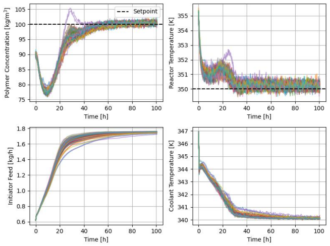
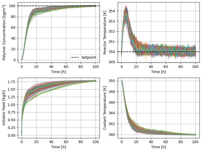
- [§6.1, Figures 5 and 6] The rollout comparisons in Figures 5 and 6 report no numerical aggregates or statistical tests, and the shaded regions overlap substantially; the claimed differences in stability and gradient direction should be quantified.
- [§4.3, Table 3] The statement that the PICNN and standard NN were trained 'using the same parameters and architecture' is ambiguous, since the PICNN imposes additional structural constraints; clarify whether the comparison uses identical layer counts, widths, and parameter counts.
Circularity Check
No significant circularity: the PICNN action-correction layer is a model-based optimizer over an explicitly defined setpoint-error cost; evaluation and cost are aligned by design, and the paper's self-citations are background only.
full rationale
The paper's derivation chain is self-contained: reactor dynamics (Eqs. 15-19) are independent ODEs; the PI-generated offline datasets, BC and IQL training (Sec. 4.1-4.2), and PICNN cost training (Sec. 4.3) follow standard supervised/offline-RL pipelines. The deployment update (Eq. 24, a_{k+1} = a_k - eta * grad_a c_hat_phi(s,a_k)) descends the learned PICNN cost model; this is model-based action optimization, not a fitted input renamed as a prediction. It is true that the evaluation reward (Eq. 20-22) is built from the same setpoint-error terms that define the cost (Eq. 23: c_t = |e_t^CP| + |e_t^T|), and the paper explicitly says the cost is 'tightly aligned with operational safety and long-term control objectives.' This is deliberate objective alignment, not circularity: the environment reward/cost used in evaluation is computed from the simulator, not from the PICNN's own output, so measured improvements are not forced by construction—indeed Figure 4 shows the PICNN has materially worse pointwise fit (R^2 = 0.73 vs 0.99), so its rollout benefit is an empirical finding. Self-citations ([2], [28], [38]) are background references and are not load-bearing for the central claim; no uniqueness theorem or unverified prior claim is imported to forbid alternatives. Two correctness/verification gaps should be noted separately from circularity: the paper never specifies whether the PICNN label paired with (s_t, a_t) is c_t or c_{t+1}, which matters for whether grad_a c_hat_phi is causally meaningful (Eq. 23 vs Eq. 24), and Section 3.3.2's 'analogous to a Lyapunov function' is asserted without a verified Lyapunov inequality. Neither gap makes the derivation circular: they are missing evidence or unspecified implementation details, not reductions of a prediction to its own input.
Assumptions & free parameters
free parameters (5)
- Gradient correction step size eta =
not reported; tuned on rollouts
- Thermal runaway threshold in reward =
e_T < -50 K (Eq. 20)
- Measurement noise magnitude =
not reported
- IQL expectile and AWR temperature =
tau = 0.9, beta = 5
- Correction clipping or projection bounds =
unspecified
assumptions (5)
- domain assumption The ODE model (Eqs. 15-19) with Table 1 parameters accurately represents a polymerisation CSTR in all three scenarios.
- domain assumption The cost c_t = |e_CP| + |e_T| is an adequate proxy for operational safety and stability, analogous to a Lyapunov function.
- standard math A PICNN that is convex in the action has a unique global minimum for each state, making gradient descent a reliable corrector.
- domain assumption The PI-generated offline datasets provide sufficient state-action coverage for BC and IQL to learn a policy that generalizes across all scenarios.
- ad hoc to paper Gradient descent on the learned PICNN cost surface improves safety in deployment without retraining or environment interaction.
Cite this review
Pith. "Pith review of Safe Deployment of Offline Reinforcement Learning via Input Convex Action Correction." pith.science (2026). https://pith.science/paper/BO4C7TIW
@misc{pith2026250722640,
  author       = {Pith},
  title        = {Pith review of: Safe Deployment of Offline Reinforcement Learning via Input Convex Action Correction},
  year         = {2026},
  howpublished = {\url{https://pith.science/paper/BO4C7TIW}},
  note         = {Machine review of arXiv:2507.22640}
}
read the original abstract
Offline reinforcement learning (offline RL) offers a promising framework for developing control strategies in chemical process systems using historical data, without the risks or costs of online experimentation. This work investigates the application of offline RL to the safe and efficient control of an exothermic polymerisation continuous stirred-tank reactor. We introduce a Gymnasium-compatible simulation environment that captures the reactor's nonlinear dynamics, including reaction kinetics, energy balances, and operational constraints. The environment supports three industrially relevant scenarios: startup, grade change down, and grade change up. It also includes reproducible offline datasets generated from proportional-integral controllers with randomised tunings, providing a benchmark for evaluating offline RL algorithms in realistic process control tasks. We assess behaviour cloning and implicit Q-learning as baseline algorithms, highlighting the challenges offline agents face, including steady-state offsets and degraded performance near setpoints. To address these issues, we propose a novel deployment-time safety layer that performs gradient-based action correction using input convex neural networks (PICNNs) as learned cost models. The PICNN enables real-time, differentiable correction of policy actions by descending a convex, state-conditioned cost surface, without requiring retraining or environment interaction. Experimental results show that offline RL, particularly when combined with convex action correction, can outperform traditional control approaches and maintain stability across all scenarios. These findings demonstrate the feasibility of integrating offline RL with interpretable and safety-aware corrections for high-stakes chemical process control, and lay the groundwork for more reliable data-driven automation in industrial systems.
Figures


Figures from the paper (21 more)






Reference graph
Works this paper leans on
-
[1]
Reinforcement Learning: An Introduction,
R. S. Sutton and A. Barto, “Reinforcement Learning: An Introduction,” 2018
work page 2018
-
[2]
From automated to autonomous process operations,
M. Baldea, A. T. Georgiou, B. Gopaluni, M. Mercang¨ oz, C. C. Pantelides, K. Sheth, V. M. Zavala, and C. Georgakis, “From automated to autonomous process operations,” Computers & Chemical Engineer- ing, vol. 196, p. 109064, 2025
work page 2025
-
[3]
Concrete Problems in AI Safety,
D. Amodei, C. Olah, J. Steinhardt, P. Christiano, J. Schulman, and D. Man´ e, “Concrete Problems in AI Safety,” 2016. [Online]. Available: https://arxiv.org/abs/1606.06565
arXiv 2016
-
[4]
Optimal grade transition for polyethylene reactors via NCO tracking,
D. Bonvin, L. Bodizs, and B. Srinivasan, “Optimal grade transition for polyethylene reactors via NCO tracking,” Chemical Engineering Research and Design, vol. 83, no. 6, pp. 692–697, 2005
work page 2005
-
[5]
K. S. Lee and J. H. Lee, “Iterative learning control-based batch process control technique for integrated control of end product properties and transient profiles of process variables,”Journal of Process Control, vol. 13, no. 7, pp. 607–621, 2003
work page 2003
-
[6]
A. Prata, J. Oldenburg, A. Kroll, and W. Marquardt, “Integrated scheduling and dynamic optimization of grade transitions for a continuous polymerization reactor,” Computers & Chemical Engineering, vol. 32, no. 3, pp. 463–476, 2008
work page 2008
-
[7]
The general problem of the stability of motion,
A. M. Lyapunov, “The general problem of the stability of motion,” International Journal of Control, vol. 55, no. 3, pp. 531–534, 1992
work page 1992
-
[8]
H. K. Khalil and J. W. Grizzle, Nonlinear Systems, 3rd ed. Prentice Hall, 1996
work page 1996
Show all 40 references
-
[9]
Input Convex Neural Networks,
B. Amos, L. Xu, and J. Z. Kolter, “Input Convex Neural Networks,” 2017. [Online]. Available: https://arxiv.org/abs/1609.07152 23
2017 arXiv
-
[10]
Safe Model-based Reinforcement Learning with Stability Guarantees,
F. Berkenkamp, M. Turchetta, A. P. Schoellig, and A. Krause, “Safe Model-based Reinforcement Learning with Stability Guarantees,” 2017. [Online]. Available: https://arxiv.org/abs/1705.08551
2017 arXiv
-
[11]
Control Barrier Function Based Quadratic Pro- grams for Safety Critical Systems,
A. D. Ames, X. Xu, J. W. Grizzle, and P. Tabuada, “Control Barrier Function Based Quadratic Pro- grams for Safety Critical Systems,” IEEE Transactions on Automatic Control, vol. 62, no. 8, pp. 3861– 3876, 2017
2017
-
[12]
Safe and Stable RL (S2RL) Driving Policies Using Control Barrier and Control Lyapunov Functions,
B. Gangopadhyay, P. Dasgupta, and S. Dey, “Safe and Stable RL (S2RL) Driving Policies Using Control Barrier and Control Lyapunov Functions,” IEEE Transactions on Intelligent Vehicles, vol. 8, no. 2, pp. 1889–1899, 2023
2023
-
[13]
Constrained Policy Optimization,
J. Achiam, D. Held, A. Tamar, and P. Abbeel, “Constrained Policy Optimization,” 2017. [Online]. Available: https://arxiv.org/abs/1705.10528
2017 arXiv
-
[14]
Safe Exploration in Continuous Action Spaces,
G. Dalal, K. Dvijotham, M. Vecerik, T. Hester, C. Paduraru, and Y. Tassa, “Safe Exploration in Continuous Action Spaces,” 2018. [Online]. Available: https://arxiv.org/abs/1801.08757
2018 arXiv
-
[15]
Conservative Q-Learning for Offline Reinforcement Learning,
A. Kumar, A. Zhou, G. Tucker, and S. Levine, “Conservative Q-Learning for Offline Reinforcement Learning,” 2020. [Online]. Available: https://arxiv.org/abs/2006.04779
2020 arXiv
-
[16]
Offline Reinforcement Learning with Implicit Q-Learning,
I. Kostrikov, A. Nair, and S. Levine, “Offline Reinforcement Learning with Implicit Q-Learning,” 2021. [Online]. Available: https://arxiv.org/abs/2110.06169
2021 arXiv
-
[17]
MOPO: Model-based Offline Policy Optimization,
T. Yu, G. Thomas, L. Yu, S. Ermon, J. Zou, S. Levine, C. Finn, and T. Ma, “MOPO: Model-based Offline Policy Optimization,” 2020. [Online]. Available: https://arxiv.org/abs/2005.13239
2020 arXiv
-
[18]
Actor–Critic Physics-Informed Neural Lyapunov Con- trol,
J. Wang and M. Fazlyab, “Actor–Critic Physics-Informed Neural Lyapunov Con- trol,” IEEE Control Systems Letters , vol. 8, p. 1751–1756, 2024. [Online]. Available: http://dx.doi.org/10.1109/LCSYS.2024.3416235
2024
-
[19]
Distributional Reinforcement Learning with Quantile Regression,
W. Dabney, M. Rowland, M. G. Bellemare, and R. Munos, “Distributional Reinforcement Learning with Quantile Regression,” 2017. [Online]. Available: https://arxiv.org/abs/1710.10044
2017 arXiv
-
[20]
EKG-AC: A New Paradigm for Process Indus- trial Optimization Based on Offline Reinforcement Learning With Expert Knowledge Guidance,
D. Liu, Y. Wang, C. Liu, B. Luo, and B. Huang, “EKG-AC: A New Paradigm for Process Indus- trial Optimization Based on Offline Reinforcement Learning With Expert Knowledge Guidance,” IEEE Transactions on Cybernetics, pp. 1–11, 2025
2025
-
[21]
Optimal Control Via Neural Networks: A Convex Approach,
Y. Chen, Y. Shi, and B. Zhang, “Optimal Control Via Neural Networks: A Convex Approach,” 2019. [Online]. Available: https://arxiv.org/abs/1805.11835
2019 arXiv
-
[22]
Differentiable Convex Optimization Layers,
A. Agrawal, B. Amos, S. Barratt, S. Boyd, S. Diamond, and Z. Kolter, “Differentiable Convex Optimization Layers,” 2019. [Online]. Available: https://arxiv.org/abs/1910.12430
2019 arXiv
-
[23]
OptNet: Differentiable Optimization as a Layer in Neural Networks,
B. Amos and J. Z. Kolter, “OptNet: Differentiable Optimization as a Layer in Neural Networks,”
-
[24]
Polymer grade transition control using advanced real-time optimization software,
S. BenAmor, F. J. Doyle III, and R. McFarlane, “Polymer grade transition control using advanced real-time optimization software,” Journal of Process Control, vol. 14, no. 4, pp. 349–364, 2004
2004
-
[25]
Polymer grade transition control via reinforcement learning trained with a physically consistent memory sequence-to-sequence digital twin,
Z.-F. Jiang, D. S.-H. Wong, J.-L. Kang, Y. Yao, and Y.-C. Chuang, “Polymer grade transition control via reinforcement learning trained with a physically consistent memory sequence-to-sequence digital twin,” in Computer Aided Chemical Engineering. Elsevier, 2023, vol. 52, pp. 297–303
2023
-
[26]
A benchmark environment motivated by industrial control problems,
D. Hein, S. Depeweg, M. Tokic, S. Udluft, A. Hentschel, T. A. Runkler, and V. Sterzing, “A benchmark environment motivated by industrial control problems,” in 2017 IEEE Symposium Series on Computa- tional Intelligence (SSCI), 2017, pp. 1–8
2017
-
[27]
Benchmarking Safe Exploration in Deep Reinforcement Learning,
A. Ray, J. Achiam, and D. Amodei, “Benchmarking Safe Exploration in Deep Reinforcement Learning,” 2019. [Online]. Available: https://arxiv.org/abs/1910.01708 24
2019 arXiv
-
[28]
PC-Gym: Benchmark Environments For Process Control Problems,
M. Bloor, J. Torraca, I. O. Sandoval, A. Ahmed, M. White, M. Mercang¨ oz, C. Tsay, E. A. D. R. Chanona, and M. Mowbray, “PC-Gym: Benchmark Environments For Process Control Problems,” arXiv preprint arXiv:2410.22093, 2024
2024 arXiv
-
[29]
End-to-End Safe Reinforcement Learning through Barrier Functions for Safety-Critical Continuous Control Tasks,
R. Cheng, G. Orosz, R. M. Murray, and J. W. Burdick, “End-to-End Safe Reinforcement Learning through Barrier Functions for Safety-Critical Continuous Control Tasks,” 2019. [Online]. Available: https://arxiv.org/abs/1903.08792
2019 arXiv
-
[30]
Offline reinforcement learning methods for real-world problems,
T. Kim, H. Suk, and S. Kim, “Offline reinforcement learning methods for real-world problems,” in Advances in Computers. Elsevier, 2024, vol. 134, pp. 285–315
2024
-
[31]
Offline reinforcement learning: Tutorial, review, and perspectives on open problems,
S. Levine, A. Kumar, G. Tucker, and J. Fu, “Offline reinforcement learning: Tutorial, review, and perspectives on open problems,” arXiv preprint arXiv:2005.01643, 2020
2005 arXiv
-
[32]
A survey on offline reinforcement learning: Taxonomy, review, and open problems,
R. F. Prudencio, M. R. Maximo, and E. L. Colombini, “A survey on offline reinforcement learning: Taxonomy, review, and open problems,” IEEE Transactions on Neural Networks and Learning Systems, 2023
2023
-
[33]
Stabilizing off-policy q-learning via bootstrapping error reduction,
A. Kumar, J. Fu, M. Soh, G. Tucker, and S. Levine, “Stabilizing off-policy q-learning via bootstrapping error reduction,” Advances in neural information processing systems, vol. 32, 2019
2019
-
[34]
Deep Reinforcement Learning with Double Q-learning,
H. van Hasselt, A. Guez, and D. Silver, “Deep Reinforcement Learning with Double Q-learning,” 2015. [Online]. Available: https://arxiv.org/abs/1509.06461
2015 arXiv
-
[35]
Human-level control through deep reinforcement learning,
V. Mnih, K. Kavukcuoglu, D. Silver, A. A. Rusu, J. Veness, M. G. Bellemare, A. Graves, M. Riedmiller, A. K. Fidjeland, G. Ostrovski et al., “Human-level control through deep reinforcement learning,”nature, vol. 518, no. 7540, pp. 529–533, 2015
2015
-
[36]
Behavior Regularized Offline Reinforcement Learning,
Y. Wu, G. Tucker, and O. Nachum, “Behavior Regularized Offline Reinforcement Learning,” 2019. [Online]. Available: https://arxiv.org/abs/1911.11361
2019 arXiv
-
[37]
Advantage-Weighted Regression: Simple and Scalable Off-Policy Reinforcement Learning,
X. B. Peng, A. Kumar, G. Zhang, and S. Levine, “Advantage-Weighted Regression: Simple and Scalable Off-Policy Reinforcement Learning,” 2019. [Online]. Available: https://arxiv.org/abs/1910.00177
2019 arXiv
-
[38]
Comparative Study of Machine Learning and System Identification for Process Systems Engineering Dynamics,
A. Ahmed, E. A. del Rio-Chanona, and M. Mercang¨ oz, “Comparative Study of Machine Learning and System Identification for Process Systems Engineering Dynamics,” Industrial & Engineering Chemistry Research, 2025
2025
-
[39]
Polymerization reactor control using autoregressive-plus Volterra- based MPC,
B. R. Maner and F. J. Doyle III, “Polymerization reactor control using autoregressive-plus Volterra- based MPC,” AIChE Journal, vol. 43, no. 7, pp. 1763–1784, 1997. 25 A Startup scenario results Figure 13: 100 PI controlled episodes from the polymerisation CSTR startup scenari...
1997
-
[2021]
Available: https://arxiv.org/abs/1703.00443
[Online]. Available: https://arxiv.org/abs/1703.00443
Reviewed August 6, 2026 · model on record in the stance chip above.
Discussion (0). Sign in to comment.