Mass-Conserving Physics-Informed Neural Networks For The One-Dimensional Advection-Diffusion Equation
Reviewed by Pith T0 review T1 audit T2 compute T3 formal T4 kernel 2026-07-08 16:45 UTCglm-5.2pith:BP47KSDZrecord.jsonopen to challenge →
The pith
Neural Net Solver Gets Mass Conservation Right at 5% Cost
A machine-rendered reading of the paper's core claim, the machinery that carries it, and where it could break.
Core claim
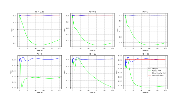
The long-term accuracy degradation in Vanilla PINNs for conservative transport is shown to be predominantly caused by the accumulation of mass drift, not by an inability to learn the spatial profile. By introducing a soft penalty term that forces the network to preserve the global integral of the concentration field, the Mass-Penalty PINN effectively eliminates this drift, restricting mass deviation to under 0.5% and stabilizing the L2 error on the order of 10^-3 over extended integration horizons.
What carries the argument
Mass-Penalty PINN: A physics-informed neural network augmented with a loss term that penalizes the squared difference between the analytically computed initial mass and the network's predicted spatial integral of mass at each time step, computed via Gaussian quadrature.
If this is right
- Mass-penalty constraints could be applied to other conservative PDEs (e.g., Navier-Stokes, Maxwell's equations) to improve long-term stability of neural network solvers.
- The finding that local PDE residuals are insufficient for global conservation suggests a broader redesign of PINN loss functions to include integral invariants by default.
- For inverse problems where analytical mass is unknown, empirically estimated mass from data could potentially substitute the analytical target, though this remains untested in the paper.
- The 5.4% training overhead suggests that adding conservation constraints is computationally cheap relative to the accuracy gains, making it a practical add-on for existing PINN implementations.
Load-bearing premise
The mass-penalty term relies on knowing the exact initial total mass from an analytical solution, which would be unavailable in inverse problems or real-world scenarios without a known ground truth.
What would settle it
If a PINN trained with the mass-penalty constraint on a long-horizon advection-diffusion problem still exhibited mass drift comparable to the Vanilla PINN (e.g., >10% mass loss), the central claim would be falsified.
Figures



read the original abstract
The advection-diffusion equation is a fundamental model of transport phenomena in which mass conservation is an essential physical constraint. While classical schemes such as Crank-Nicolson preserve this property by construction, Physics-Informed Neural Networks (PINNs) enforce only the local residual of the governing PDE and are therefore not guaranteed to conserve global quantities such as mass over long integration horizons. In this work, we examine the extent of this limitation for the periodic one-dimensional advection-diffusion equation and evaluate a Mass-Penalty PINN that augments the standard PINN loss with a soft mass-conservation constraint. We compare the performance of Vanilla PINN, Mass-Penalty PINN, and the Crank-Nicolson scheme across a range of Peclet numbers spanning diffusion-dominated to advection-dominated regimes, and over two simulation horizons representing short-term and long-term dynamics. The results show that, for short-term simulations, the Mass-Penalty PINN does not always provide a consistent improvement in accuracy. However, for long-term simulations, the Mass-Penalty PINN reduces the relative L2 error and mass conservation error by factors of approximately 9-67 and 15-215, respectively, compared with the Vanilla PINN, across the tested Peclet numbers. Further analysis reveals that the accuracy degradation observed in Vanilla PINN is predominantly caused by the accumulation of mass drift over time. These results demonstrate that incorporating a soft mass-conservation constraint substantially improves the long-term reliability of PINN for conservative transport problems, particularly in mitigating mass drift over extended simulation horizons.
Editorial analysis
A structured set of objections, weighed in public.
Referee Report
Summary. This manuscript evaluates a Mass-Penalty PINN for the 1D advection-diffusion equation, comparing it against a Vanilla PINN and a Crank-Nicolson baseline across seven Peclet numbers (0.01–20) and two time horizons (T=5 s, T=100 s). The mass-penalty approach augments the standard PINN loss with a soft constraint penalizing deviation from the analytically known initial mass. The central claim is that for long-term simulations (T=100 s), the Mass-Penalty PINN reduces relative L2 error by 9–67× and mass conservation error by 15–215× compared to Vanilla PINN, at a training cost increase of only 5.4%. The experimental design is reasonable: the Peclet range spans diffusion- to advection-dominated regimes, an analytical reference solution is available, and a grid-independence study establishes the CN baseline.
Significance. The paper addresses a practically relevant problem—mass drift in PINNs over long integration horizons—and provides a systematic sweep over Peclet numbers that is uncommon in the PINN literature. The use of an analytical reference solution and a grid-verified CN baseline is a strength. The mass-penalty approach itself is not novel (it follows [28]), but its systematic evaluation for advection-diffusion transport across flow regimes fills a documented gap. The computational cost analysis (Table 1) is a useful addition. However, the quantitative claims rest on experimental results whose statistical robustness is not established, which limits the significance of the reported improvement factors.
major comments (2)
- §2.5, §3.2: All quantitative results (improvement factors of 9–67× for L2 error and 15–215× for mass error) appear to be from single training runs. No error bars, standard deviations, or number of random seeds are reported anywhere in the manuscript. PINN training is stochastic: network initialization, LHS collocation point sampling, and optimizer trajectories all vary across seeds. The headline improvement factors are presented as deterministic ranges, but without variance estimates it is impossible to assess whether the lower bounds (9×, 15×) are reproducible or whether they could collapse for specific Peclet numbers. This is load-bearing for the central claim. At minimum, the authors should report results averaged over multiple seeds (≥3–5) with standard deviations for each Peclet number and time horizon, and revise the improvement-factor claims accordingly.
- §2.5: The penalty weights (λ_IC=100, λ_BC=20, λ_PDE=10, λ_m=10) were established via a 'preliminary hyperparameter tuning study' citing [29] (DeepXDE). It is unclear whether this tuning was performed with the mass penalty active or for the Vanilla configuration only. If the weights were optimized with the mass penalty on, the Vanilla PINN baseline may be using suboptimal hyperparameters, which would inflate the apparent improvement. The authors should clarify which configuration was used during tuning, and ideally confirm that the Vanilla baseline uses its own optimized weights. Additionally, the sensitivity of results to λ_m=10 is not reported; a brief sensitivity analysis (e.g., λ_m ∈ {1, 10, 100}) would strengthen the claim that a single fixed λ_m is robust across all Peclet numbers.
minor comments (7)
- §2.4, Eq. (8): The notation switches between L_m and L_mass (§3.1 uses 'Lmass constraint with λmass = 10'). Standardize on one notation.
- §2.4, Eq. (9): The Gaussian quadrature rule used for the mass integral is not specified (number of points, order). Since this integral is evaluated at every training step and its accuracy directly affects the mass-penalty term, the quadrature details should be stated.
- §2.4: Reference [26] (and possibly [?]) appears with a question mark in the reference list, indicating a missing citation. Please fix.
- §3.1: The statement that the Mass-Penalty PINN 'slightly underperforms' Vanilla in diffusion-dominated short-term runs is qualitative. Quantifying the difference (e.g., relative L2 error values for Pe=0.01 at T=5 s for both methods) would help the reader assess the tradeoff.
- Figures 3–7: The axis labels and legends are small and difficult to read. Consider enlarging font sizes and ensuring line styles/colors are distinguishable in print.
- §3.3, Table 1: The CN inference time (≈3.03 s) is not directly comparable to PINN inference time because CN solves the full spatio-temporal grid while the PINN evaluates at queried points. A brief note clarifying what 'inference' means for each method would improve fairness of the comparison.
- §5: The conclusion states the mass penalty reduces errors 'by up to 67 and 215 times,' but the abstract and §3.2 report ranges (9–67, 15–215). Ensure consistency in phrasing.
Simulated Author's Rebuttal
We thank the referee for a careful and constructive report. Both major comments are well-taken and address genuine gaps in the experimental rigor of the manuscript. We address each below.
read point-by-point responses
-
Referee: §2.5, §3.2: All quantitative results appear to be from single training runs. No error bars, standard deviations, or number of random seeds are reported. PINN training is stochastic. The headline improvement factors are presented as deterministic ranges, but without variance estimates it is impossible to assess whether the lower bounds (9×, 15×) are reproducible. At minimum, report results averaged over multiple seeds (≥3–5) with standard deviations for each Peclet number and time horizon, and revise the improvement-factor claims accordingly.
Authors: The referee is correct. All results in the current manuscript are from single training runs, and no variance estimates are reported. This is a genuine weakness in the experimental design, and we agree that the improvement factors (9–67× for L2 error, 15–215× for mass error) cannot be reliably interpreted without knowing the spread across random seeds. We will revise the manuscript to include results averaged over at least 5 random seeds for every Peclet number and both time horizons, reporting mean ± standard deviation for both the relative L2 error and the mass conservation error. We will also recompute and revise the improvement-factor ranges accordingly, reporting them as mean improvement factors with appropriate uncertainty rather than as deterministic bounds. If any Peclet number shows high variance that undermines the lower-bound claims, we will state this explicitly rather than reporting only the favorable cases. The abstract and conclusions will be updated to reflect the revised, statistically grounded claims. revision: yes
-
Referee: §2.5: The penalty weights were established via a 'preliminary hyperparameter tuning study' citing [29] (DeepXDE). It is unclear whether this tuning was performed with the mass penalty active or for the Vanilla configuration only. If the weights were optimized with the mass penalty on, the Vanilla PINN baseline may be using suboptimal hyperparameters, which would inflate the apparent improvement. Clarify which configuration was used during tuning, and ideally confirm that the Vanilla baseline uses its own optimized weights. Additionally, the sensitivity of results to λ_m=10 is not reported; a brief sensitivity analysis (e.g., λ_m ∈ {1, 10, 100}) would strengthen the claim that a single fixed λ_m is robust across all Peclet numbers.
Authors: We acknowledge that the manuscript is unclear on this point. In the current version, the penalty weights (λ_IC=100, λ_BC=20, λ_PDE=10) were tuned on the Vanilla PINN configuration first, and then λ_m=10 was selected separately for the Mass-Penalty PINN. However, this procedure was not documented in the manuscript, and the referee is right that the lack of clarity raises the concern that the Vanilla baseline may be disadvantaged (or, conversely, that the Mass-Penalty configuration was not jointly optimized). We will revise §2.5 to explicitly state the tuning protocol. In the revised manuscript, we will also conduct and report a separate hyperparameter tuning for the Vanilla PINN to confirm that its weights are not suboptimal. Regarding the sensitivity to λ_m: the referee's suggestion is reasonable and we agree it strengthens the robustness claim. We will add a sensitivity analysis for λ_m ∈ {1, 10, 100} across representative Peclet numbers (at minimum Pe = 0.01, 1, 20) for the long-term horizon, reporting both L2 and mass errors. If the results show that λ_m=10 is not robust across all regimes, we will report this honestly and discuss regime-dependent choices. revision: yes
Circularity Check
No significant circularity: the mass-penalty target is an externally computed analytical invariant, and the improvement factors are measured against an independent baseline.
full rationale
The paper's central result is that adding a soft mass-conservation penalty to a PINN loss function improves long-term accuracy and mass conservation compared to a Vanilla PINN. Walking the derivation chain: (1) The target mass m(c_0) = Aσ√(2π) (Eq. 6) is derived analytically from the initial condition (Eq. 3) via the Method of Images solution (Eq. 5). This is an externally computable invariant of the PDE, not a quantity defined in terms of the PINN's own output. (2) The mass-penalty loss L_m (Eq. 8) penalizes the network's predicted mass m(c_θ, t_i) (Eq. 9, computed via Gaussian quadrature) against this analytical target. The penalty is a soft constraint, not a hard redefinition — the network can still violate mass conservation, and the paper reports residual mass errors of 0.08–0.43%. (3) The improvement factors (9–67× for L2, 15–215× for mass error) are computed by comparing the Mass-Penalty PINN against the Vanilla PINN baseline, both evaluated against the same analytical reference solution (Eq. 5). Neither the metrics nor the baseline is defined in terms of the method being tested. (4) The mass-penalty strategy is attributed to Huang et al. [28] (external citation, Cahn-Hilliard context), not a self-citation. (5) The hyperparameter tuning reference [29] is to DeepXDE (Lu et al.), an external library, not the authors' own prior work. The only minor concern is that λ_m = 10 was tuned on the same benchmark setup, but this is a standard hyperparameter selection issue (a correctness/statistical concern), not circularity — the penalty weight does not determine the analytical mass target or the evaluation metric by construction. The derivation is self-contained against external benchmarks.
Axiom & Free-Parameter Ledger
free parameters (8)
- λ_IC =
100
- λ_BC =
20
- λ_PDE =
10
- λ_m =
10
- Network architecture =
4 layers × 50 neurons
- N_interior =
20000
- N_IC =
4000
- N_BC =
4000
axioms (5)
- standard math The 1D advection-diffusion equation with periodic boundary conditions conserves total mass.
- standard math The analytical solution via the Method of Images (Eq. 5) is exact for the periodic domain.
- domain assumption The tanh activation function produces sufficiently smooth outputs for automatic differentiation of the PDE residual.
- domain assumption Gaussian quadrature with the chosen number of nodes accurately approximates the spatial integral of the neural network output for the mass penalty.
- ad hoc to paper A single set of penalty weights (λ_IC=100, λ_BC=20, λ_PDE=10, λ_m=10) is optimal across all seven Peclet numbers and both time horizons.
Reference graph
Works this paper leans on
-
[1]
Abdul Qadir Mugheri. Efficient explicit numerical technique for modeling advection diffusion reaction for a water quality model in an opened uniform flow – a 1d perspective.Journal of Mechanics of Continua and Mathematical Sciences, 2023
work page 2023
-
[2]
Y . E. Aghdam, H. Mesgrani, M. Javidi, and O. Nikan. A computational approach for the space-time fractional advection–diffusion equation arising in contaminant transport through porous media.Engineering with Computers, 37:3615–3627, 2020
work page 2020
-
[3]
Romuald Szymkiewicz and Dariusz G ˛ asiorowski. Adaptive method for the solution of 1d and 2d advec- tion–diffusion equations used in environmental engineering.Journal of Hydroinformatics, 23(6):1290–1311, 2021
work page 2021
-
[4]
Physical Informed Neural Networks for modeling ocean pollutant
Karishma Battina, Prathamesh Joshi, Raj Dandekar, Rajat Dandekar, and Sreedath Panat. Physical informed neural networks for modeling ocean pollutant.arXiv preprint arXiv:2507.08834, 2025
work page internal anchor Pith review Pith/arXiv arXiv 2025
-
[5]
Jiayi Xie, Hongfeng Li, Shaoyi Su, Jin Cheng, Qingrui Cai, Hanbo Tan, Lingyun Zu, Xiaobo Qu, and Hongbin Han. Quantitative analysis of molecular transport in the extracellular space using physics-informed neural network. Computers in Biology and Medicine, 171:108133, 2024
work page 2024
-
[6]
AirPhyNet: Harnessing Physics-Guided Neural Networks for Air Quality Prediction
Kethmi Hirushini Hettige, Jiahao Ji, Shili Xiang, Cheng Long, Gao Cong, and Jingyuan Wang. Airphynet: Harnessing physics-guided neural networks for air quality prediction.arXiv preprint arXiv:2402.03784, 2024
work page internal anchor Pith review Pith/arXiv arXiv 2024
-
[7]
LeVeque.Finite Volume Methods for Hyperbolic Problems
Randall J. LeVeque.Finite Volume Methods for Hyperbolic Problems. Cambridge University Press, 2002
work page 2002
-
[8]
Finite volume methods.Handbook of Numerical Analysis, 7:731–1018, 2000
Robert Eymard, Thierry Gallouët, and Raphaële Herbin. Finite volume methods.Handbook of Numerical Analysis, 7:731–1018, 2000
work page 2000
-
[9]
J. Crank and P. Nicolson. A practical method for numerical evaluation of solutions of partial differential equations of the heat-conduction type.Mathematical Proceedings of the Cambridge Philosophical Society, 43(1):50–67, 1947
work page 1947
-
[10]
W. Hundsdorfer and J. G. Verwer.Numerical Solution of Time-Dependent Advection-Diffusion-Reaction Equations. Springer, 2003
work page 2003
- [11]
-
[12]
Atilim G. Baydin, Barak A. Pearlmutter, Alexey A. Radul, and Jeffrey M. Siskind. Automatic differentiation in machine learning: a survey.Journal of Machine Learning Research, 18:1–43, 2018
work page 2018
-
[13]
George E. Karniadakis, Ioannis G. Kevrekidis, Lu Lu, Paris Perdikaris, Sifan Wang, and Liu Yang. Physics- informed machine learning.Nature Reviews Physics, 3:422–440, 2021
work page 2021
-
[14]
di Cola, Fabio Giampaolo, Gianluigi Rozza, Maziar Raissi, and Francesco Piccialli
Salvatore Cuomo, Vincenzo S. di Cola, Fabio Giampaolo, Gianluigi Rozza, Maziar Raissi, and Francesco Piccialli. Scientific machine learning through physics-informed neural networks: Where we are and what’s next.Journal of Scientific Computing, 92(3):88, 2022
work page 2022
-
[15]
Shengze Cai, Zhiping Mao, Zhicheng Wang, Minglang Yin, and George E. Karniadakis. Physics-informed neural networks (pinns) for fluid mechanics: a review.Acta Mechanica Sinica, 37(12):1727–1738, 2021. 8 APREPRINT- JULY8, 2026
work page 2021
-
[16]
Krishnapriyan, Asghar Gholami, Shandian Zhe, Robert M
Aditi S. Krishnapriyan, Asghar Gholami, Shandian Zhe, Robert M. Kirby, and Michael W. Mahoney. Character- izing possible failure modes in physics-informed neural networks.Advances in Neural Information Processing Systems, 34, 2021
work page 2021
-
[17]
M. L. Mamud, M. K. Mudunuru, S. Karra, and B. Ahmmed. Quantifying local and global mass balance errors in physics-informed neural networks.Scientific Reports, 14(1):15541, 2024
work page 2024
-
[18]
Sifan Wang, Yujun Teng, and Paris Perdikaris. Understanding and mitigating gradient flow pathologies in physics-informed neural networks.SIAM Journal on Scientific Computing, 43(5):A3055–A3081, 2021
work page 2021
-
[19]
Sifan Wang, Xinling Yu, and Paris Perdikaris. When and why pinns fail to train: A neural tangent kernel perspective.Journal of Computational Physics, 449:110768, 2022
work page 2022
-
[20]
Ameya D. Jagtap and George E. Karniadakis. Extended physics-informed neural networks (xpinns): A generalized space-time domain decomposition based deep learning framework for nonlinear partial differential equations. Communications in Computational Physics, 28(5):2002–2041, 2020
work page 2002
-
[21]
Jagtap, Ehsan Kharazmi, and George E
Ameya D. Jagtap, Ehsan Kharazmi, and George E. Karniadakis. Conservative physics-informed neural networks on discrete domains for conservation laws: Applications to forward and inverse problems.Computer Methods in Applied Mechanics and Engineering, 365:113028, 2020
work page 2020
-
[22]
Khemraj Shukla, Ameya D. Jagtap, and George E. Karniadakis. Parallel physics-informed neural networks via domain decomposition.Journal of Computational Physics, 447:110683, 2021
work page 2021
-
[23]
Ehsan Kharazmi, Zhongqiang Zhang, and George E.M. Karniadakis. hp-vpinns: Variational physics-informed neural networks with domain decomposition.Computer Methods in Applied Mechanics and Engineering, 374:113547, 2021
work page 2021
-
[24]
Finite Volume Neural Network: Modeling Subsurface Contaminant Transport
Timothy Praditia, Matthias Karlbauer, Sebastian Otte, Sergey Oladyshkin, Martin V . Butz, and Wolfgang Nowak. Finite volume neural network: Modeling subsurface contaminant transport.arXiv preprint arXiv:2104.06010, 2021
work page internal anchor Pith review Pith/arXiv arXiv 2021
-
[25]
Nathan Lichtlé, Alexi Canesse, Zhe Fu, Hossein Nick Zinat Matin, Maria Laura Delle Monache, and Alexandre M. Bayen. (u)nfv: Supervised and unsupervised neural finite volume methods for solving hyperbolic pdes.arXiv preprint arXiv:2505.23702, 2025
work page internal anchor Pith review Pith/arXiv arXiv 2025
-
[26]
Coupled integral pinn for conservation law.arXiv preprint arXiv:2411.11276, 2024
Yeping Wang and Shihao Yang. Coupled integral pinn for conservation law.arXiv preprint arXiv:2411.11276, 2024
-
[27]
Patsatzis, Mario di Bernardo, Lucia Russo, and Constantinos Siettos
Dimitrios G. Patsatzis, Mario di Bernardo, Lucia Russo, and Constantinos Siettos. Gorinns: Godunov-riemann in- formed neural networks for learning hyperbolic conservation laws.Journal of Computational Physics, 534:114002, 2025
work page 2025
-
[28]
Qiumei Huang, Jiaxuan Ma, and Zhen Xu. Mass-preserving spatio-temporal adaptive pinn for cahn-hilliard equations with strong nonlinearities and singularities.Preprint submitted to Elsevier, 2025
work page 2025
-
[29]
DeepXDE: A deep learning library for solving differential equations
Lu Lu, Xuhui Meng, Zhiping Mao, and George E. Karniadakis. Deepxde: A deep learning library for solving differential equations.arXiv preprint arXiv:1907.04502, 2019
work page internal anchor Pith review Pith/arXiv arXiv 1907
-
[30]
Lu Lu, Pengzhan Jin, Guofei Pang, Zhongqiang Zhang, and George E. Karniadakis. Learning nonlinear operators via deeponet based on the universal approximation theorem of operators.Nature Machine Intelligence, 3:218–229, 2021
work page 2021
-
[31]
Kovachki, Kamyar Azizzadenesheli, Burigede Liu, Kaushik Bhattacharya, Andrew M
Zong-Yi Li, Nikola B. Kovachki, Kamyar Azizzadenesheli, Burigede Liu, Kaushik Bhattacharya, Andrew M. Stuart, and Anima Anandkumar. Fourier neural operator for parametric partial differential equations.International Conference on Learning Representations, 2021
work page 2021
-
[32]
Zongyi Li, Hongkai Zheng, Nikola Kovachki, David Jin, Haoxuan Chen, Burigede Liu, Kamyar Azizzadenesheli, and Anima Anandkumar. Physics-informed neural operator for learning partial differential equations.ACM / IMS Journal of Data Science, 1, 2021
work page 2021
-
[33]
Rambod Mojgani, Maciej Balajewicz, and Pedram Hassanzadeh. Kolmogorov n–width and lagrangian physics- informed neural networks: A causality-conforming manifold for convection-dominated pdes.Computer Methods in Applied Mechanics and Engineering, 404:115810, 2023
work page 2023
-
[34]
Jeremy Yu, Lu Lu, Xuhui Meng, and George E. Karniadakis. Gradient-enhanced physics-informed neural networks for forward and inverse pde problems.Computer Methods in Applied Mechanics and Engineering, 393:114823, 2022
work page 2022
-
[35]
Matthias Karlbauer, Timothy Praditia, Sebastian Otte, Sergey Oladyshkin, Wolfgang Nowak, and Martin V . Butz. Composing partial differential equations with physics-aware neural networks.arXiv preprint arXiv:2111.11798, 2022. 9 APREPRINT- JULY8, 2026
work page internal anchor Pith review Pith/arXiv arXiv 2022
-
[36]
Chenxi Wu, Min Zhu, Qinyang Tan, Yadhu Kartha, and Lu Lu. A comprehensive study of non-adaptive and residual-based adaptive sampling for physics-informed neural networks.arXiv preprint arXiv:2207.10289, 2022. 10
work page internal anchor Pith review Pith/arXiv arXiv 2022
discussion (0)
Sign in with ORCID, Apple, or X to comment. Anyone can read and Pith papers without signing in.