REVIEW 4 major objections 6 minor 19 references
Mass Estimation from Images using Deep Neural Network and Sparse Ground Truth
T0 review · 4 major / 6 minor · reviewed 2026-08-14 · deepseek-v4-flash
Pith's one-line read A deep network can estimate flowing material mass from images using only one total-mass label per run, reaching 95.5% test-set accuracy and beating a calibrated stereo-volume baseline.
desk verdict Useful engineering paper whose headline accuracy number is run-level; the per-frame mass-flow claim is not actually demonstrated, but the core aggregation idea and honest volume-baseline comparison make it worth serious refereeing. read the letter →
The pith
A machine-rendered reading of the paper's core claim, the machinery that carries it, and where it could break.
The reading
What carries the argument
The load-bearing object is the sparse-ground-truth aggregation loss. For a run $i$ with total mass $y_i$ and images $x_{ij}$ captured at speed $v_{ij}$ and fixed time step $t$, the loss is $L_i = \frac{1}{n_i}(y_i - \sum_{j=1}^{n_i} f(x_{ij};w) v_{ij} t)^2 + \frac{\lambda}{n_i}\sum_{j=1}^{n_i}(f(x_{ij};w) - f(x_{i(j-1)};w))^2$. The first term converts one per-run scale reading into a training signal for every image; the second penalizes frame-to-frame jumps to stabilize the predicted mass signal. A gradient-accumulation procedure keeps the summed gradients, predictions, and smoothing terms in memory across batches, so runs with too many images for GPU memory can still be trained in full.
What would settle it
Take the same elevator and camera rig, run test loads across speeds from near zero to normal operating speed, and compare each run's scale-measured total mass with the model's speed-scaled summed prediction. If the summed prediction deviates systematically at low speeds or under speed fluctuations—as it did for the paper's own outlier run—the velocity-scaling assumption is false and the reported accuracy will not transfer.
Extended reading notes
Core claim
The central claim is that a DNN trained on images with only one scalar label per run—the total load weight—can learn to estimate the mass contribution of each frame. The loss compares the sum of speed- and time-scaled per-image predictions against the run's total mass, so the sparse label is spread across every image by backpropagation. With a temporal-smoothness penalty added, the 9-layer residual network RES-9ER reaches 95.5% test-set accuracy, and the predicted signal is more stable and accurate than the volume-based signal in incremental, intermittent, and poor-lighting flow scenarios. The paper argues the network captures the density physics of randomly stacked slender rods internally, removing the need for the explicit density calibration that the stereo-volume method requires.
Load-bearing premise
The load-bearing premise is that a run's measured total mass equals the sum of per-image mass predictions after multiplying each by elevator speed and capture time, which assumes the speed signal is accurate and every frame's material is counted exactly once.
Editorial extensions
If this is right
- Harvester mass-flow sensing could be built from a 2-D camera plus speed signal, dropping stereo point clouds and density calibration.
- Any process that records only batch totals—grain loads, conveyor runs, truckloads—becomes trainable without per-item labels, provided the speed/time scaling holds.
- Temporal smoothing adds a small but consistent accuracy gain (about 0.6% on average across architectures) and visibly smoother predictions, which helps real-time control.
- The 45,921-parameter RES-9ER network is small enough for embedded devices, so the method can run on the machine itself.
Reading between the lines
- An implication the authors leave implicit: the method inherits its accuracy from the speed signal; their own low-speed outlier shows the first thing to break on a real harvester will be the velocity-scaling assumption, not the image model.
- Since the aggregation term sums frames without regard to order, a shuffled-frame training experiment would isolate how much of the reported gain comes from the physics-based scaling versus the temporal-smoothing penalty.
- The comparison with volume estimates excludes low-light runs for the volume baseline, so a fair read is that the DNN gains come partly from learned density and partly from not needing minimum lighting; a controlled illumination sweep could separate those effects.
- The same total-label trick should transfer to other conserved quantities measured from video—total counts of animals, vehicles, or defects from sequence-level totals—whenever a linear accumulation assumption with a known proportionality signal holds.
Signed reviews
Editorial analysis
A structured set of objections, weighed in public.
Referee Report
Summary. The paper proposes a semi-supervised deep learning method for estimating mass flow of material (bamboo surrogate for sugarcane) on an elevator from 2D images, using only run-level total mass labels. The training loss in Eq. (3) compares the sum of per-image predictions (scaled by elevator speed and capture time) to the run total, augmented by a temporal smoothness penalty. The authors report test accuracy up to 95.5% for a 9-layer residual network (RES-9ER) with temporal smoothing, claim it surpasses a calibrated stereo-volume baseline, and present grad-CAM visualizations, an architecture reduction analysis, and a memory-efficient gradient accumulation algorithm for long image sequences.
Significance. If the empirical claims are substantiated with proper validation, the method is practically valuable: it replaces a calibrated stereo-volume system with a commodity 2D camera and offers a general template for regression with sparse labels via an aggregated loss. The paper includes open-source code, an explicit loss formulation, and a clear statement of the speed-scaling assumption. The main theoretical novelty is a simple reformulation of MSE loss for aggregated labels rather than a new learning paradigm, but the application is meaningful and the reported qualitative signal improvements are plausible. The current strength of the claims, however, exceeds what the defined metrics actually support.
major comments (4)
- [Section 3.2, Eq. (3) and Table 2] The 'Test-Set Accuracy' in Table 2 is never defined, and the loss in Eq. (3) supervises only the run-level sum of predictions. Because the first term of Eq. (3) is invariant to zero-sum rearrangements of per-frame predictions, a model that outputs a constant per-frame flow equal to the run average can achieve the same run-level loss as a model that correctly tracks within-run flow. The abstract and Section 4.2 explicitly claim 'mass flow estimation' and display per-frame signal plots, so the authors must provide per-frame or segment-level errors (e.g., RMSE over short time windows) to show that the learned per-image predictions are meaningful. Without such validation, the 95.5% figure supports only run-total mass prediction, not the stated mass-flow claim.
- [Section 4.4] The low-speed outlier (average speed 0.1 m/s with large variations) is acknowledged as a failure in which the DNN used sidewall reflections to compensate for a low-fidelity speed signal. This is not merely a corner-case artifact; it is a direct consequence of the aggregate loss, where the run-level target can be satisfied by exploiting spurious cues that correct for speed error. The manuscript dismisses the outlier as unlikely in practice, but the operational speed range over which the method is reliable is never characterized. A robustness analysis across speed ranges, or a demonstration with a higher-fidelity speed sensor, is needed to bound the envelope in which the load-bearing speed-scaling assumption holds.
- [Section 4.3 and Table 2] The claimed superiority over the volume-based method is not quantitatively supported. Table 2 reports accuracies only for the DNN architectures; the global accuracy of the volume-based baseline is never tabulated. Section 4.3 relies on visual inspection of Figures 8 and 9b ('can be seen to perform much better'), and Figure 9b is a histogram without numerical error statistics. The authors should report the volume baseline's error on the same test-set metric, the same test runs, and the same exclusion rules (e.g., low-light runs excluded for volume), so that the abstract's claim of surpassing volumetric methods can be verified.
- [Section 3.3, Eq. (4)] The gradient equation is not self-contained: the symbol '˙y' (breve) is used without definition, and the temporal term in Eq. (4) does not correspond to the loss term in Eq. (3), which is defined on f(x_{ij};w) rather than on the speed-corrected prediction used elsewhere. As written, Eq. (4) cannot be verified against Eq. (3) or Algorithm 1, which matters because the memory-efficient gradient accumulation procedure is a stated contribution of the work.
minor comments (6)
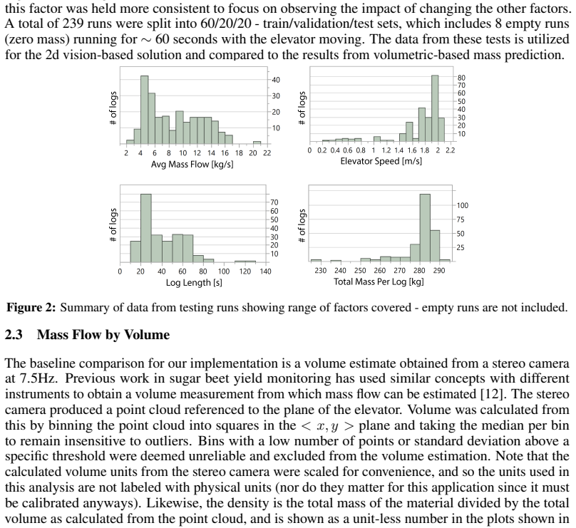
- [Section 2.2] Please clarify whether the 8 empty runs are included in the train/validation/test split and how they are treated in the reported accuracy, since zero-mass runs may behave differently from loaded runs.
- [Section 2.1, Eq. (1)] The normalization term 'n' in Eq. (1) lacks the run index; it should be 'n_i' to match Eq. (3), where the run length appears as n_i.
- [Section 3.2] The temporal smoothing weight λ is stated as 'chosen empirically 0.05'; please describe the selection procedure or provide a small sensitivity analysis to show that the result is not strongly dependent on this value.
- [Figure 7 and Section 4.2] The caption refers to 'RunX' without defining which run it is, and the statement 'improved accuracy by 6.6% and 2.8%' does not specify which accuracy measure is used; please clarify the metric and the baseline in both places.
- [Algorithm 1] The symbols '⊕' and '˙' and the notation 'ŷbgrad' are not defined in the main text or the algorithm; please introduce them explicitly before use.
- [References] Reference [19] contains a malformed date '2019-74-21'; the access date should be corrected.
Circularity Check
No circularity: the run-level loss uses external ground truth, and no load-bearing claim reduces to its own input.
full rationale
The central derivation is self-contained against external ground truth. Equation 3 supervises the sum of per-image, speed-scaled predictions against the run-level total mass label, L_i = (1/n_i)(y_i - sum_j f(x_ij;w) v_ij t)^2 + lambda-term. This is a genuine weakly supervised regression loss: the target y_i is an external measurement, not a function of the network's own output, and held-out test runs provide an independent check. Nothing in the loss defines the prediction in terms of the fitted parameter; rather, the network must generalize to unseen runs to score well in Table 2. The volume-based baseline in Eq. 2 is fitted with its own density network, but it is only a comparison method and its fitted parameters are not renamed as the paper's prediction. The temporal smoothing term and architecture choices (RES-9ER, ELU, reduced filters) are standard empirical model selection, tuned on validation behavior rather than defined by the target. The only self-referential element is the mention of 'previous unpublished work of our own' for the experimental design, which is not load-bearing for the mass-prediction claim. The identifiability concern that run-level supervision does not uniquely constrain per-frame mass flow is a real correctness/validity risk, but it is not circularity: a model that collapses to the run average would still need to match held-out run totals, and the paper's qualitative signal plots and grad-cam analyses are additional, if incomplete, evidence. Under the stated rubric, no step reduces Eq. 3 to its own inputs or imports a load-bearing result solely from self-citation, so the appropriate circularity score is 0.
Assumptions & free parameters
free parameters (3)
- Temporal smoothing weight lambda =
0.05
- Volume baseline density network parameters theta and bias beta =
not reported
- DNN architecture hyperparameters for RES-9ER =
45,921 parameters
assumptions (5)
- domain assumption Total run mass equals the sum of per-image mass contributions after scaling by elevator speed and capture time (additivity over frames).
- domain assumption The speed sensor provides accurate velocity for every frame across the operating range.
- domain assumption The fixed camera and elevator geometry make mass a learnable function of 2D images, with no unobserved material.
- domain assumption Bamboo under controlled testing is a valid surrogate for harvested sugarcane, so density physics and visual patterns transfer.
- domain assumption First-order temporal differences in predicted mass are a valid smoothness prior.
Cite this review
Pith. "Pith review of Mass Estimation from Images using Deep Neural Network and Sparse Ground Truth." pith.science (2026). https://pith.science/paper/BRIXWAPX
@misc{pith2026190804387,
  author       = {Pith},
  title        = {Pith review of: Mass Estimation from Images using Deep Neural Network and Sparse Ground Truth},
  year         = {2026},
  howpublished = {\url{https://pith.science/paper/BRIXWAPX}},
  note         = {Machine review of arXiv:1908.04387}
}
read the original abstract
Supervised learning is the workhorse for regression and classification tasks, but the standard approach presumes ground truth for every measurement. In real world applications, limitations due to expense or general in-feasibility due to the specific application are common. In the context of agriculture applications, yield monitoring is one such example where simple-physics based measurements such as volume or force-impact have been used to quantify mass flow, which incur error due to sensor calibration. By utilizing semi-supervised deep learning with gradient aggregation and a sequence of images, in this work we can accurately estimate a physical quantity (mass) with complex data structures and sparse ground truth. Using a vision system capturing images of a sugarcane elevator and running bamboo under controlled testing as a surrogate material to harvesting sugarcane, mass is accurately predicted from images by training a DNN using only final load weights. The DNN succeeds in capturing the complex density physics of random stacking of slender rods internally as part of the mass prediction model, and surpasses older volumetric-based methods for mass prediction. Furthermore, by incorporating knowledge about the system physics through the DNN architecture and penalty terms, improvements in prediction accuracy and stability, as well as faster learning are obtained. It is shown that the classic nonlinear regression optimization can be reformulated with an aggregation term with some independence assumptions to achieve this feat. Since the number of images for any given run are too large to fit on typical GPU vRAM, an implementation is shown that compensates for the limited memory but still achieve fast training times. The same approach presented herein could be applied to other applications like yield monitoring on grain combines or other harvesters using vision or other instrumentation.
Figures


Figures from the paper (6 more)


Reference graph
Works this paper leans on
-
[1]
An introduction to machine learning
Pierre Lison. An introduction to machine learning. Springer: Berlin, Germany, 2015
work page 2015
-
[2]
Machine learning: an algorithmic perspective
Stephen Marsland. Machine learning: an algorithmic perspective. Chapman, 2011
work page 2011
-
[3]
Semi-supervised elastic net for pedestrian counting
Ben Tan, Junping Zhang, and Liang Wang. Semi-supervised elastic net for pedestrian counting. Pattern Recognition, 44(10):2297–2304, 2011
work page 2011
-
[4]
Maria Pérez-Ortiz, JM Peña, Pedro Antonio Gutiérrez, Jorge Torres-Sánchez, César Hervás- Martínez, and Francisca López-Granados. A semi-supervised system for weed mapping in sunflower crops using unmanned aerial vehicles and a crop row detection method. Applied Soft Computing, 37:533–544, 2015
work page 2015
-
[5]
Semi-supervised deep learning for monocular depth map prediction
Yevhen Kuznietsov, Jorg Stuckler, and Bastian Leibe. Semi-supervised deep learning for monocular depth map prediction. In Proceedings of the IEEE Conference on Computer Vision and Pattern Recognition, pages 6647–6655, 2017
work page 2017
-
[6]
Watch and learn: Semi-supervised learning for object detectors from video
Ishan Misra, Abhinav Shrivastava, and Martial Hebert. Watch and learn: Semi-supervised learning for object detectors from video. In Proceedings of the IEEE Conference on Computer Vision and Pattern Recognition, pages 3593–3602, 2015
work page 2015
-
[7]
V olumetric mass flow sensor for citrus mechanical harvesting machines
U Jadhav, LR Khot, R Ehsani, V Jagdale, and JK Schueller. V olumetric mass flow sensor for citrus mechanical harvesting machines. Computers and electronics in agriculture, pages 93–101, 1993
work page 1993
-
[8]
JUNSU Shin. Mass and Size Estimation of citrus Fruit by Machine vision and citrus greening diseased fruit detection using spectral analysis. PhD thesis, University of Florida, 2012
work page 2012
Show all 19 references
-
[9]
Mass-flow estimation in mineral-processing applications
Teemu Väyrynen, Pekka Itävuo, Matti Vilkko, Antti Jaatinen, and Mika Peltonen. Mass-flow estimation in mineral-processing applications. IFAC Proceedings, 46(16):271–276, 2013
2013
-
[10]
Introduction to semi-supervised learning
Xiaojin Zhu and Andrew B Goldberg. Introduction to semi-supervised learning. Synthesis lectures on artificial intelligence and machine learning, 3(1):1–130, 2009
2009
-
[11]
Policy gradient methods for reinforcement learning with function approximation
Richard S Sutton, David A McAllester, Satinder P Singh, and Yishay Mansour. Policy gradient methods for reinforcement learning with function approximation. In Advances in neural information processing systems, pages 1057–1063, 2000
2000
-
[12]
In-Soil Measuring of Sugar Beet Yield Using UWB Radar Sensor System
Miodrag Konstantinovic et al. In-Soil Measuring of Sugar Beet Yield Using UWB Radar Sensor System. PhD thesis, Universitäts-und Landesbibliothek Bonn, 2007
2007
-
[13]
Evolutions of packing properties of perfect cylinders under densification and crystallization
Lufeng Liu, Ye Yuan, Wei Deng, and Shuixiang Li. Evolutions of packing properties of perfect cylinders under densification and crystallization. The Journal of chemical physics , 149(10):104–503, 2018
2018
-
[14]
Experimental and computational analysis of random cylinder packings with applications
Wenli Zhang. Experimental and computational analysis of random cylinder packings with applications. PhD thesis, Louisiana State University, 2006
2006
-
[15]
Neural machine translation by jointly learning to align and translate
Dzmitry Bahdanau, Kyunghyun Cho, and Yoshua Bengio. Neural machine translation by jointly learning to align and translate. arXiv preprint arXiv:1409.0473, 2014
2014 arXiv
-
[16]
Identity mappings in deep residual networks
Kaiming He, Xiangyu Zhang, Shaoqing Ren, and Jian Sun. Identity mappings in deep residual networks. In European conference on computer vision, pages 630–645. Springer, 2016
2016
-
[17]
Image analysis and comparison
James Cryer and the Huddle development team. Image analysis and comparison. https: //github.com/rsmbl/Resemble.js, 2018. Accessed: 2019-04-28
2018
-
[18]
Grad-cam++: Generalized gradient-based visual explanations for deep convolutional networks
Aditya Chattopadhay, Anirban Sarkar, Prantik Howlader, and Vineeth N Balasubramanian. Grad-cam++: Generalized gradient-based visual explanations for deep convolutional networks. In 2018 IEEE Winter Conference on Applications of CV (WACV), pages 839–847. IEEE, 2018
2018
-
[19]
Eager execution in tensorflow
Tensorflow team. Eager execution in tensorflow. https://www.tensorflow.org/guide/ eager, 2019. Accessed: 2019-74-21. 9
2019
Reviewed August 14, 2026 · model on record in the stance chip above.
Discussion (0). Continue with ORCID to comment.