REVIEW 2 major objections 6 minor 49 references
Measuring the Algorithmic Convergence of Randomized Ensembles: The Regression Setting
T0 review · 2 major / 6 minor · reviewed 2026-08-14 · deepseek-v4-flash
Pith's one-line read The paper establishes that resampling an ensemble's own trained functions yields a bootstrap quantile that serves as an approximately valid conditional upper bound on the gap between a finite ensemble's error and its infinite-ensemble…
desk verdict A genuinely useful bootstrap for regression ensemble convergence, with a real theorem and a clearly named gap between the proved result and the implemented algorithm. read the letter →
The pith
A machine-rendered reading of the paper's core claim, the machinery that carries it, and where it could break.
The reading
What carries the argument
The identity $\mathrm{mse}_t - \mathrm{mse}_{\infty} = \psi(\overline{T}_t) - \psi(\vartheta)$, where $\psi(f) = \int (y - f(x))^2 \, d\nu$ is the mean-squared-error functional, $\overline{T}_t$ is the ensemble average, and $\vartheta(x) = E[\overline{T}_t(x) \mid D]$ is its conditional expectation over algorithmic randomness. The identity converts the unobservable gap between a finite average and its limit into a difference of a smooth functional at two averages, so that resampling the trained functions $T_1,\ldots,T_t$ with replacement and forming $\mathrm{mse}^*_t - \mathrm{mse}_t = \psi(\overline{T}^{\,*}_t) - \psi(\overline{T}_t)$ produces bootstrap samples whose $(1-\alpha)$-quantile mimics the target quantile. The load-bearing proof ingredients are a Rosenthal-type moment inequality for sums of independent Banach-valued random variables, which controls the residual $\|\overline{T}_t - \vartheta\|^2_{L^2}$; a Berry\textendash Esseen (quantitative central limit) bound chaining the standardized pivot to a Gaussian; and the Dvoretzky\textendash Kiefer\textendash Wolfowitz inequality (the standard uniform deviation bound for empirical distributions) chaining the bootstrap empirical quantile to its conditional distribution.
What would settle it
Fix a training set $D$, run many independent ensembles on the same $D$, and compare the empirical frequency of $\mathrm{mse}_t - \mathrm{mse}_{\infty} \le \hat q_{1-\alpha}(t)$ with the predicted level $1-\alpha - c_0\delta_{t,k,B}(D)$, under all three implementations: the theoretical bootstrap using the exact functional $\psi$, Algorithm 1 with a hold-out set of size $m$, and Algorithm 1 with out-of-bag predictions. If the theoretical version covers at the predicted level but the practical versions fall short precisely when $m$ or the effective out-of-bag size is small, the missing $\widehat\psi$-error bound is the cause; if the practical versions fail even with $\psi$ known, the Gaussian and moment approximations in the proof are at fault.
Extended reading notes
Core claim
The central claim is Theorem 3.1. For any randomized regression ensemble satisfying the representation $T_i = \phi(x; D, \xi_i)$ with i.i.d. randomizing parameters $\xi_i$ given the training data $D$, and under a mild moment assumption, the empirical $(1-\alpha)$-quantile $\hat q_{1-\alpha}(t)$ of $B$ bootstrap samples of the form $\mathrm{mse}^*_t - \mathrm{mse}_t$ satisfies $$P\big(\mathrm{mse}_t - \mathrm{mse}_{\infty} \le \hat q_{1-\$\alpha$}(t) \mid D\big) \ge 1 - \$\alpha$ - c_0\delta_{t,k,B}(D),$$ where $\delta_{t,k,B}(D) = \frac{k^2}{\sqrt{t}}\left(\frac{\beta_{3k}(D)}{\sigma(D)}\right)^3 + e^{-k/2} + \sqrt{\frac{\log B}{B}}$. In words, the bootstrap quantile is an approximately valid conditional upper confidence bound on the convergence gap between the finite ensemble and the ideal infinite ensemble, with an explicit non-asymptotic bound on the coverage error. The proof approximates $\sqrt{t}(\mathrm{mse}_t - \mathrm{mse}_{\infty})$ by a Gaussian with variance $\sigma^2(D)$, approximates the bootstrap pivot by a Gaussian with the resampled variance, and shows the two variances are close; each step is controlled by a Banach-space moment inequality, a Berry\textendash Esseen (quantitative central limit) bound, and the Dvoretzky\textendash Kiefer\textendash Wolfowitz inequality. When the base learner is CART (the standard greedy regression-tree algorithm) or any method whose predictions stay within the range of the training labels, choosing $k \approx \log t - 4\log\log t$ reduces the bound to $c(D)\frac{\log^2 t}{\sqrt{t}} + \sqrt{\frac{\log B}{B}}$, i.e., nearly parametric decay.
Load-bearing premise
The coverage guarantee in Theorem 3.1 is proved only for bootstrap samples built from the true error functional $\psi$, while the implemented Algorithm 1 and all experiments use an estimate $\widehat\psi$ from hold-out or out-of-bag samples, so the practical guarantee rests on the unproven premise that this estimation error is negligible, which can fail when the hold-out set is small or the effective out-of-bag size is small.
Editorial extensions
If this is right
- A practitioner who runs bagging or random forests once on a fixed data set can compute the bootstrap quantile from the stored predicted values alone and obtain an upper bound, certified up to an explicit coverage error, on how far the finite ensemble's error is from the infinite-ensemble error at any chosen level.
- Because the coverage error is non-asymptotic and shrinks at nearly parametric rates in both the ensemble size and the number of bootstrap replications, the guarantee has bite at finite ensemble sizes, not merely in the limit of infinitely many trees.
- The extrapolation rule, based on the gap scaling as one over the square root of the ensemble size, lets a small initial ensemble predict the size needed to bring the gap within a chosen tolerance; when out-of-bag estimates are used, the effective ensemble size (the expected number of out-of-bag trees per training point) must be substituted, and the paper shows this bias correction is what makes th
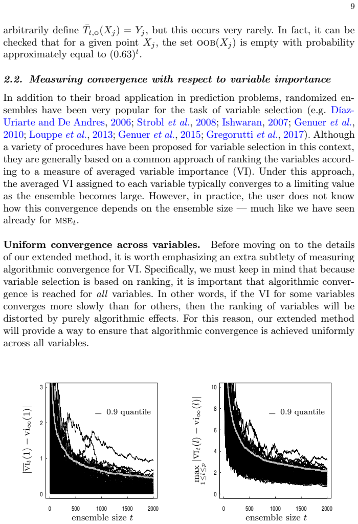
- Applied to variable importance, the same resampling certifies that every variable's importance score has converged uniformly, so that rankings compare variables fairly rather than reflecting algorithmic noise on slow-converging variables.
- The computational cost of the convergence check is on the order of the number of bootstrap samples times the ensemble size times the validation size, which is no larger than the cost of training the trees when the number of bootstrap samples is modest; the variable-importance variant is independent of the sample size and highly scalable.
Reading between the lines
- A natural next theorem, which the paper leaves open, would prove a matching guarantee for the estimated error functional, tracking the hold-out size or the out-of-bag effective size explicitly so that the coverage error picks up a term on the order of one over the square root of that size; the numerics suggest the out-of-bag version's larger effective sample is why it outperforms the small hold-ou
- The one-sided quantile could support two-sided confidence statements about the infinite-ensemble error itself, since the same Gaussian approximation of the standardized gap that drives the proof should also yield intervals around the limit.
- For data sets with very many variables, the worst-case importance deviation should grow like the square root of the log-variable-count over the ensemble size under the bootstrap; the method already handles this automatically, but the same machinery could predict how much of an observed spread in importance scores is purely algorithmic.
- Because the method consumes only predicted values, it transfers to any randomized estimator with a convergent average, such as Bayesian additive regression trees, random rotations, or random projections, which the paper lists as within scope of its abstract representation but does not test.
Signed reviews
Editorial analysis
A structured set of objections, weighed in public.
Referee Report
Summary. The paper proposes a bootstrap method for deciding whether a randomized regression ensemble (bagging, random forests) is large enough. For a fixed training set D, it targets the (1−α)-quantile q_{1−α}(t) of the convergence gap mse_t − mse∞, where mse_t is the conditional test MSE of the averaged ensemble and mse∞ is its limit. Algorithm 1 resamples the t trained functions with replacement and uses the empirical quantile of ψ̂(T̅*_t) − ψ̂(T̅_t) as an estimator, with ψ estimated from hold-out or out-of-bag samples. Theorem 3.1 gives a non-asymptotic conditional coverage bound for the corresponding oracle bootstrap that uses the true functional ψ; Section 2.2 extends the idea to variable importance; Section 4 analyzes cost and proposes 1/√t extrapolation with an out-of-bag bias correction; Section 5 contains experiments on four datasets.
Significance. The oracle-bootstrap result is a genuine contribution if it stands: under assumptions A1–A2 it gives an explicit, non-asymptotic rate δ_{t,k,B}(D) → 0 in t and B, with only mild moment conditions, and the supplementary proof is detailed and uses standard tools (Talagrand/Rosenthal inequalities, DKW, Berry–Esseen). The CART moment bound in Eq. (3.3) and the cost comparison in Section 4.1 are also useful. However, the main theorem is proven only for bootstrap samples constructed from the unknown functional ψ, whereas Algorithm 1 and every numerical result use an estimated ψ̂; no result controls the estimation error. This gap is central to the paper's advertised practical claim and must be addressed in revision.
major comments (2)
- [Section 3, Eq. (3.5); Section 2, Algorithm 1, Eqs. (2.5)–(2.7)] Theorem 3.1 is stated for q̂_{1−α}(t) defined as the empirical quantile of B bootstrap samples of the form (2.5), i.e. ψ(T̅*_t) − ψ(T̅_t) with the true functional ψ. The text at the beginning of Section 3 explicitly says the analysis focuses on bootstrap samples that are 'not affected by the extraneous error from estimating the functional ψ.' But Algorithm 1 and all experiments use z_{t,b} := ψ̂(T̅*_t) − ψ̂(T̅_t) with ψ̂ from (2.6) or (2.7). The manuscript contains no result bounding the difference between the empirical quantiles of these two bootstrap distributions, or the difference in coverage. At the numerical operating point (t0 = 500, B = 50, hold-out fraction ≈ 1/6, oob effective size ≈ 0.37 t0), the estimation error is not a priori negligible. Because the abstract and Section 1 present the bootstrap as a practical method, this is a load-bearing gap, not a cosmetic one.
- [Section 4.2, Eqs. (4.2) and (4.4); Section 5.2] The estimators plotted and recommended in Section 5 are the extrapolated oob estimator (4.4) and the hold-out estimator (4.2). Both rely on the heuristic q_{1−α}(t) ≈ κ/√t, and no theorem or quantitative bound is given for the error of this approximation or for the coverage of the extrapolated interval. Thus even a proof of Theorem 3.1 for the non-extrapolated ψ̂-based estimator would not justify the headline numerical claim that the method predicts convergence at t = 2,000 from t0 = 500. The paper should either prove, under stated assumptions, a bound on the extrapolation error, or explicitly mark the extrapolation as a heuristic and restrict the formal claims to the non-extrapolated estimate.
minor comments (6)
- [Section 1] There are small typos: 'The purpose of the current paper is develop a solution' should be 'is to develop a solution,' and 'has not beaddressed' in Section 1.2 should be 'has not been addressed.'
- [Section 3 and Section 2] The same symbol q̂_{1−α}(t) is used for the empirical quantile of the oracle bootstrap in Theorem 3.1 and for the output of Algorithm 1 with estimated ψ̂; these are different estimators and the notation should be distinguished.
- [Section 4.2, Eq. (4.3)] τ_n(t0) is defined as the expected cardinality of oob(X_j), but it is then called the 'effective' ensemble size; since the oob set is random, the text should make clear that q_{1−α}(τ_n(t0)) is an approximation based on an expectation.
- [Section 5.1] The 'true' quantile curves are approximations: they come from 1,000 runs, with mse_{2,000} used as a surrogate for mse∞. This approximation should be stated more prominently near the figures, not only in the experimental setup.
- [Section 2.2, Algorithm 2] No theoretical guarantee is stated for the variable-importance bootstrap; if this is meant as an empirical extension, the text should say so explicitly.
- [Section 5.2] The error bars in Figures 3–6 are 10th and 90th percentiles over runs; the text says they are not confidence intervals, but a brief explanation of what they do represent would improve clarity.
Circularity Check
No significant circularity: the bootstrap coverage theorem is a standalone non-asymptotic proof, and self-citations are methodological rather than load-bearing.
full rationale
The central claim (Theorem 3.1) is proven from scratch in the supplementary material using standard external inequalities (Talagrand's Rosenthal inequality, Dvoretzky-Kiefer-Wolfowitz, Berry-Esseen) and does not fit any parameter to data. The target object is q1−α(t), the conditional quantile of mse_t − mse_infinity, while the bootstrap samples are independently defined in equation (2.5) as ψ(T̄*_t) − ψ(T̄_t); these are not equal by construction, and the theorem's proof bounds their distributional distance. The citation to Lopes (2019) supplies only the general resampling template and the 1/√t extrapolation heuristic; the regression-specific result and its error bounds are new and self-contained. The well-known gap between the theory (true functional ψ) and Algorithm 1 (estimated ψ̂) is explicitly acknowledged in Section 3 and is a limitation, not a circular step: no equation is redefined as its own input and no fitted value is renamed as a prediction. Consequently, the analysis is not circular.
Assumptions & free parameters
assumptions (6)
- domain assumption Ensemble functions T_i admit representation (1.2), i.e., they are conditionally i.i.d. given D (Assumption A1).
- domain assumption Moment condition beta_{3k}(D) < infinity for some k >= 2 (Assumption A2).
- standard math Talagrand's inequality for independent Banach-valued random variables (Lemma D.1).
- standard math Dvoretzky-Kiefer-Wolfowitz inequality and Berry-Esseen bounds hold for the relevant conditional distributions.
- domain assumption The test point distribution nu is fixed and independent of D and xi_t; the functional psi is treated as known in the theoretical guarantee.
- ad hoc to paper The quantile q_{1-alpha}(t) scales like kappa / sqrt(t) (Section 4.2).
Cite this review
Pith. "Pith review of Measuring the Algorithmic Convergence of Randomized Ensembles: The Regression Setting." pith.science (2026). https://pith.science/paper/CKRCDLWU
@misc{pith2026190801251,
  author       = {Pith},
  title        = {Pith review of: Measuring the Algorithmic Convergence of Randomized Ensembles: The Regression Setting},
  year         = {2026},
  howpublished = {\url{https://pith.science/paper/CKRCDLWU}},
  note         = {Machine review of arXiv:1908.01251}
}
read the original abstract
When randomized ensemble methods such as bagging and random forests are implemented, a basic question arises: Is the ensemble large enough? In particular, the practitioner desires a rigorous guarantee that a given ensemble will perform nearly as well as an ideal infinite ensemble (trained on the same data). The purpose of the current paper is to develop a bootstrap method for solving this problem in the context of regression --- which complements our companion paper in the context of classification (Lopes 2019). In contrast to the classification setting, the current paper shows that theoretical guarantees for the proposed bootstrap can be established under much weaker assumptions. In addition, we illustrate the flexibility of the method by showing how it can be adapted to measure algorithmic convergence for variable selection. Lastly, we provide numerical results demonstrating that the method works well in a range of situations.
Figures


Figures from the paper (3 more)


Reference graph
Works this paper leans on
-
[1]
Arlot, S. and Genuer, R. (2014) Analysis of purely random forests bias. preprint arXiv:1407.3939
arXiv 2014
-
[2]
Basilico, J., Munson, M., Kolda, T., Dixon, K. and Kegelmeyer, W. (2011) Comet: A recipe for learning and using large ensembles on massive data. In Data Mining (ICDM), 2011 IEEE 11th International Conference on, 41--50. IEEE
work page 2011
-
[3]
(2012) Analysis of a random forests model
Biau, G. (2012) Analysis of a random forests model. Journal of Machine Learning Research, 13, 1063--1095
work page 2012
-
[4]
Biau, G., Devroye, L. and Lugosi, G. (2008) Consistency of random forests and other averaging classifiers. Journal of Machine Learning Research, 9, 2015--2033
work page 2008
-
[5]
Bickel, P. J. and Yahav, J. A. (1988) Richardson extrapolation and the bootstrap. Journal of the American Statistical Association, 83, 387--393
work page 1988
-
[6]
Blaser, R. and Fryzlewicz, P. (2016) Random rotation ensembles. The Journal of Machine Learning Research, 17, 126--151
work page 2016
-
[7]
Breiman, L. (1996) Bagging predictors. Machine Learning, 24, 123--140
work page 1996
- [8]
Show all 49 references
-
[9]
Breiman, L., Friedman, J., Stone, C. J. and Olshen, R. A. (1984) Classification and R egression T rees . CRC press
1984
-
[10]
and Zaglia, M
Brezinski, C. and Zaglia, M. R. (2013) Extrapolation Methods: theory and practice. Elsevier
2013
-
[11]
and Yu, B
B \"u hlmann, P. and Yu, B. (2002) Analyzing bagging. The Annals of Statistics, 30, 927--961
2002
-
[12]
Cannings, T. I. and Samworth, R. J. (2017) Random projection ensemble classification (with discussion). Journal of the Royal Statistical Society Series B
2017
-
[13]
A., George, E
Chipman, H. A., George, E. I., McCulloch, R. E. et al. (2010) Bart: Bayesian additive regression trees. The Annals of Applied Statistics, 4, 266--298
2010
-
[14]
and De Andres, S
D \' az-Uriarte, R. and De Andres, S. A. (2006) Gene selection and classification of microarray data using random forest. BMC bioinformatics, 7, 3
2006
-
[15]
and Graff, C
Dua, D. and Graff, C. (2017) UCI machine learning repository. ://archive.ics.uci.edu/ml
2017
-
[16]
and Wolfowitz, J
Dvoretzky, A., Kiefer, J. and Wolfowitz, J. (1956) Asymptotic minimax character of the sample distribution function and of the classical multinomial estimator. The Annals of Mathematical Statistics, 642--669
1956
-
[17]
and Tibshirani, R
Friedman, J., Hastie, T. and Tibshirani, R. (2001) The E lements of S tatistical L earning . Springer
2001
-
[18]
and Tuleau-Malot, C
Genuer, R., Poggi, J.-M. and Tuleau-Malot, C. (2010) Variable selection using random forests. Pattern Recognition Letters, 31, 2225--2236
2010
-
[19]
and Tuleau-Malot, C
Genuer, R., Poggi, J.-M. and Tuleau-Malot, C. (2015) Vsurf: an R package for variable selection using random forests. The R Journal, 7, 19--33
2015
-
[20]
(2017) Hands-on machine learning with Scikit-Learn and TensorFlow
G \'e ron, A. (2017) Hands-on machine learning with Scikit-Learn and TensorFlow. O'Reilly Media. ://github.com/ageron/handson-ml/tree/master/datasets
2017
-
[21]
and Saint-Pierre, P
Gregorutti, B., Michel, B. and Saint-Pierre, P. (2017) Correlation and variable importance in random forests. Statistics and Computing, 27, 659--678
2017
-
[22]
and Samworth, R
Hall, P. and Samworth, R. J. (2005) Properties of bagged nearest neighbour classifiers. Journal of the Royal Statistical Society: Series B, 67, 363--379
2005
-
[23]
and Su \'a rez, A
Hern \'a ndez-Lobato, D., Mart \' nez-Mu \ n oz, G. and Su \'a rez, A. (2013) How large should ensembles of classifiers be? Pattern Recognition, 46, 1323--1336
2013
-
[24]
(2007) Variable importance in binary regression trees and forests
Ishwaran, H. (2007) Variable importance in binary regression trees and forests. Electronic Journal of Statistics, 1, 519--537
2007
-
[25]
B., Schechtman, G
Johnson, W. B., Schechtman, G. and Zinn, J. (1985) Best constants in moment inequalities for linear combinations of independent and exchangeable random variables. The Annals of Probability, 234--253
1985
-
[26]
Kwapie\'n, S., Szulga, J. et al. (1991) Hypercontraction methods in moment inequalities for series of independent random variables in normed spaces. The Annals of Probability, 19, 369--379
1991
-
[27]
and Decaestecker, C
Latinne, P., Debeir, O. and Decaestecker, C. (2001) Limiting the number of trees in random forests. In Multiple Classifier Systems. Springer
2001
-
[28]
and Wiener, M
Liaw, A. and Wiener, M. (2002) Classification and regression by random F orest. R News, 2, 18--22
2002
-
[29]
and Jeon, Y
Lin, Y. and Jeon, Y. (2006) Random forests and adaptive nearest neighbors. Journal of the American Statistical Association, 101, 578--590
2006
-
[30]
Lopes, M. E. (2016) A sharp bound on the computation-accuracy tradeoff for majority voting ensembles. preprint arXiv:1303.0727
2016 arXiv
-
[31]
Lopes, M. E. (2019) Estimating the algorithmic variance of randomized ensembles via the bootstrap. The Annals of Statistics, 47, 1088--1112
2019
-
[32]
and Geurts, P
Louppe, G., Wehenkel, L., Sutera, A. and Geurts, P. (2013) Understanding variable importances in forests of randomized trees. In Advances in Neural Information Processing Systems, 431--439
2013
-
[33]
(1990) The tight constant in the D voretzky- K iefer- W olfowitz inequality
Massart, P. (1990) The tight constant in the D voretzky- K iefer- W olfowitz inequality. The Annals of Probability, 18, 1269--1283
1990
-
[34]
and Hooker, G
Mentch, L. and Hooker, G. (2016) Quantifying uncertainty in random forests via confidence intervals and hypothesis tests. Journal of Machine Learning Research, 17, 1--41
2016
-
[35]
and Tramontano, A
Moult, J., Fidelis, K., Kryshtafovych, A. and Tramontano, A. (2011) Critical assessment of methods of protein structure prediction (CASP) --- round IX . Proteins: Structure, Function, and Bioinformatics, 79, 1--5
2011
-
[36]
Ng, A. Y. and Jordan, M. I. (2001) Convergence rates of the voting G ibbs classifier, with application to B ayesian feature selection. In International Conference on Machine Learning, 377--384
2001
-
[37]
M., Perez, P
Oshiro, T. M., Perez, P. S. and Baranauskas, J. A. (2012) How many trees in a random forest? In Machine Learning and Data Mining in Pattern Recognition, 154--168. Springer
2012
-
[38]
and Boulesteix, A.-L
Probst, P. and Boulesteix, A.-L. (2018) To tune or not to tune the number of trees in random forest. Journal of Machine Learning Research, 18, 1--18
2018
-
[39]
and Pollefeys, M
Schwing, A., Zach, C., Zheng, Y. and Pollefeys, M. (2011) Adaptive random forest -- H ow many ``experts'' to ask before making a decision? In Computer Vision and Pattern Recognition (CVPR), 2011 IEEE Conference on, 1377--1384. IEEE
2011
-
[40]
(2016 a ) On the asymptotics of random forests
Scornet, E. (2016 a ) On the asymptotics of random forests. Journal of Multivariate Analysis, 146, 72--83
2016
-
[41]
(2016 b ) Random forests and kernel methods
Scornet, E. (2016 b ) Random forests and kernel methods. IEEE Transactions on Information Theory, 62, 1485--1500
2016
-
[42]
and Vert, J.-P
Scornet, E., Biau, G. and Vert, J.-P. (2015) Consistency of random forests. The Annals of Statistics, 43, 1716--1741
2015
-
[43]
and Laake, P
Sexton, J. and Laake, P. (2009) Standard errors for bagged and random forest estimators. Computational Statistics & Data Analysis, 53, 801--811
2009
-
[44]
(2003) Practical Extrapolation Methods: Theory and Applications
Sidi, A. (2003) Practical Extrapolation Methods: Theory and Applications. Cambridge University Press
2003
-
[45]
and Zeileis, A
Strobl, C., Boulesteix, A.-L., Kneib, T., Augustin, T. and Zeileis, A. (2008) Conditional variable importance for random forests. BMC bioinformatics, 9, 307
2008
-
[46]
(1989) Isoperimetry and integrability of the sum of independent B anach-space valued random variables
Talagrand, M. (1989) Isoperimetry and integrability of the sum of independent B anach-space valued random variables. The Annals of Probability, 1546--1570
1989
-
[47]
and Efron, B
Wager, S., Hastie, T. and Efron, B. (2014) Confidence intervals for random forests: the jackknife and the infinitesimal jackknife. Journal of Machine Learning Research, 15, 1625--1651
2014
-
[48]
(2016) ggplot2: Elegant Graphics for Data Analysis
Wickham, H. (2016) ggplot2: Elegant Graphics for Data Analysis. Springer-Verlag New York
2016
-
[49]
and King, R
Zhou, F., Claire, Q. and King, R. D. (2014) Predicting the geographical origin of music. In 2014 IEEE International Conference on Data Mining, 1115--1120. IEEE
2014
Reviewed August 14, 2026 · model on record in the stance chip above.
Discussion (0). Continue with ORCID to comment.