REVIEW 4 major objections 5 minor 88 references
ARIES: Relation Assessment and Model Recommendation for Deep Time Series Forecasting
T0 review · 4 major / 5 minor · reviewed 2026-08-05 · deepseek-v4-flash
Pith's one-line read ARIES claims that seven cheaply computed time series properties predict which deep forecasting model will win, backed by benchmarks of 50+ models and a parameter-free recommender.
desk verdict A genuinely useful integrated benchmark/recommender for time-series forecasting, but the headline relation claim needs statistical grounding and the synthetic-to-real transfer premise is thinner than advertised. read the letter →
The pith
A machine-rendered reading of the paper's core claim, the machinery that carries it, and where it could break.
The reading
What carries the argument
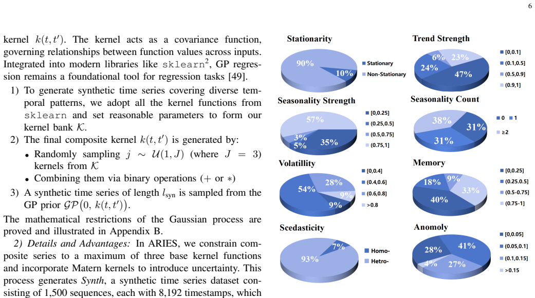
The load-bearing piece is the Synth dataset paired with the 8-bit property vector. Synth is 1,500 Gaussian-process series of 8,192 timestamps, each sampled from a composite kernel formed by randomly adding or multiplying up to three kernels from a kernel bank — a recipe that yields controllable, stable patterns with known properties. Each series' history is scored on the seven properties using standard tests (ADF/KPSS/ACF for stationarity, Mann-Kendall for trend, ACF detection with MSTL for seasonality, coefficient of variation for volatility, Hurst exponent for memorability, ARCH LM test for scedasticity, z-score proportion for anomaly) and binned into an 8-bit vector. That vector keys a st
What would settle it
Run the paper's strategy ablations (moving-average vs Fourier decomposition, RevIN on/off) on real-world series binned into the same 8-bit property intervals as Synth, using the same protocol; if the improvement signs of Table VII flip or vanish within matched bins, the synthetic-to-real transfer fails. The ETTh1 result is an early partial check — recommendation quality drops when history and future diverge — so repeating the check on other datasets with known distribution shift would bound the transfer claim.
Extended reading notes
Core claim
On the paper's own terms, the discovery is a measurable, repeatable correspondence between time series properties and modeling strategies, established by benchmarking 50+ models on a controllable synthetic dataset. Strong trends favor channel-interaction architectures and Fourier-style decomposition, while moving-average decomposition hurts them; strong and multi-seasonal series favor moving-average decomposition and deep residual learning over Fourier methods; deep models handle high volatility better than low; long-term memory separates models more than any other property, with channel strategy outweighing the transformer-versus-MLP backbone; reversible instance normalization (RevIN) yield
Load-bearing premise
The load-bearing premise is that the synthetic Synth series — random sums and products of up to three Gaussian-process kernels with hand-set parameters — reproduce the same property-to-performance relationships as real-world time series, so rankings measured on them transfer to any real series with matching property values.
Editorial extensions
If this is right
- If the property-strategy correspondence holds, practitioners can profile a new series with seven CPU-only property computations and receive a ranked model shortlist, eliminating most trial-and-error benchmarking.
- The opposite preferences of moving-average and Fourier decomposition — one favors strong seasonality, the other strong trends — make decomposition choice a data-dependent decision, and explain why mixed-pattern real benchmarks hid the effect.
- RevIN's large uniform gains make it a fairness precondition: new models should include it and comparisons should hold it fixed, otherwise reported gains may be normalization gains rather than architecture gains.
- Recommendation reliability inherits the stability of the series: on ETTh1, where history and future diverge, both fine-grained and sequence-wise accuracy drop, marking the boundary of the approach.
- Because the recommender is parameter-free, adding models or datasets only updates the key-value store, and recommendations complete in seconds to about a minute on CPU.
Reading between the lines
- Editorial inference: the paper's transfer claim is testable from inside its own design — generate a second synthetic corpus from a different family (ARIMA/state-space or Fourier-plus-STL mixtures) with the same 8-bit property-vector bins and re-check whether model rankings and the Table VII strategy preferences survive. If they flip, the GP kernel bank, not the property vector alone, shaped the fi
- Editorial inference: the per-series performance records in ARIES TEST enable a property-conditioned ensemble the paper does not propose: weight models by the property profile of each forecast window instead of recommending a single model.
- Editorial inference: the paper observes that foundation models show muted or absent property preferences (Moirai near the parameter-free baseline, no volatility bias); this suggests zero-shot foundation models and property-aware selection are complements rather than substitutes, a direction the paper reports but does not develop.
- Editorial inference: the paper flags history-future consistency as its main limitation; that suggests a concrete deployment rule it does not generalize — measure history-future similarity (as in its Figure 15) before trusting a recommendation and fall back to simple MLP baselines on low-similarity data.
Editorial analysis
A structured set of objections, weighed in public.
Referee Report
Summary. The paper proposes ARIES, a framework that (i) constructs a large synthetic time-series dataset (Synth) from Gaussian-process kernels, (ii) computes seven time-series properties (stationarity, trend, seasonality, volatility, memorability, scedasticity, anomaly) for every series, (iii) benchmarks 50+ forecasting models on Synth, and (iv) uses the resulting property-performance table to derive qualitative relations between data properties and modeling strategies, and to build a retrieval-based, parameter-free model recommender. The recommender encodes each series as an 8-bit property vector, retrieves similar Synth series, and ranks models by their mean performance on those neighbors. The paper validates the recommender on Electricity, PEMS08, and ETTh1 and reports hit-ratio/NDCG numbers. The central claim is that the experimental results reveal a clear correlation between time-series properties and modeling strategies, and that ARIES is the first study to establish these relations and to implement a deep forecasting model recommender.
Significance. If the central claim is established, ARIES would be a useful community resource: it provides a controllable synthetic benchmark, a systematic property-evaluation pipeline, a large model-strategy-per-property table, and an interpretable, low-cost recommendation procedure. The paper ships code, which is a concrete strength, and the stability analysis of the property definitions (Appendix A) is a good-practice element. However, the paper's headline claims substantially exceed what the current evidence supports. The relation assessment is qualitative (boxplots and tables) without a single correlation coefficient or significance test, and the transfer from Synth to real data is validated on only three narrow datasets whose property vectors occupy a small corner of the designed property space. These issues are load-bearing because the abstract and Section IV state the 'clear correlation' as a finding, and Section V claims a reliable recommender. Thus the paper needs major strengthening before the central claims can be accepted.
major comments (4)
- [Section IV.D, Figure 13 and Tables III–IV] The central claim of a 'clear correlation' between time-series properties and modeling strategies is supported only by qualitative inspection of boxplots and performance tables. No correlation coefficient, significance test, confidence interval, or multiple-comparison control is reported. This is load-bearing because the abstract and Section IV.D state the correlation as a finding. Please add a quantitative analysis — e.g., Spearman rank correlation between property bin levels and model error ranks, with permutation tests or corrected p-values — and report effect sizes for the claimed contrasts (e.g., moving-average vs. Fourier decomposition, high-memory vs. low-memory).
- [Section V.D, Table VI (PEMS08)] The reported metric values are internally inconsistent. For PEMS08, Hit Ratio@5_o = 0.0 but Hit Ratio@7_o = 1.0, and NDCG@5_o = 0.0 but NDCG@7_o = 0.546. If Hit Ratio@K is the standard fraction of queries with a hit in the top-K, then HR@7 must be at least HR@5 because the top-7 list contains the top-5 list. These numbers suggest the metric is not a standard hit rate — possibly a binary 'top-K lists intersect' indicator or a different aggregation. Since the paper's claim of 'overall Hit Ratio close to 1' rests on these numbers, the metric must be defined precisely and all affected results recomputed.
- [Section III.B1 and Appendix E] The synthetic-to-real transfer premise is not established. Synth is generated from at most three sklearn GP kernels combined by + or *, which yields continuous, smooth patterns; Appendix B explicitly states that discontinuous points and missing-data mutations are not represented, and Appendix E limits ARIES to 'remarkable temporal patterns' while excluding 'highly noisy and distributionally shifting data.' Yet the abstract claims a general 'clear correlation' and recommendations for 'realistic time series.' The real-data validation (Section V.D) uses only Electricity, PEMS08, and ETTh1, all non-stationary, heteroscedastic, seasonal, and low-memory — they do not exercise the property space used to build Table V (high memory, low volatility, high anomaly, etc.). The 'Synth only' substitution test only shows that one real dataset is a worse key set than Synth for another real dataset; it do
- [Section III.A, Eq. (1) and Figure 11] The stationarity definition is ambiguous. Eq. (1) claims to measure 'strictly-sense stationarity' but uses ADF, KPSS, and ACF convergence, which are wide-sense (covariance) stationarity tests; the thresholds for the ADF/KPSS decisions are not given in the equation. This matters because stationarity is one of the seven properties used both for the relation analysis and as a component of the recommender keys. In addition, the binning intervals in Figure 11 are fitted to the Synth distribution and then used both to derive property-strategy relations and to construct the recommender keys; the paper does not report robustness to these binning choices. Please clarify the definition, provide the exact thresholds, and add a sensitivity analysis for the binning.
minor comments (5)
- [Section III.A, Eq. (5)] The variable x'_i in the volatility formula is not defined. It should be clarified whether the series is detrended or transformed before computing the coefficient of variation.
- [Table VI (ETTh1)] Sumba appears both in 'Models with potential preferences' and in 'Potentially unsuitable Models' for the same dataset. This internal inconsistency should be resolved.
- [Abstract and Figure 9] There are typos: 'deep forcasting' in the abstract, 'Homo-scadasticity and Hetro-scadasticity' in Figure 9, 'Scadasticity' in Appendix A, and 'Moriai' in Section IV.D8. Please correct.
- [Algorithm 1] The condition 'p mod pi >= 2' is ambiguous when pi does not divide p. Also, the sampling frequency fs is defaulted to 1.0 but for real data this should be user-specified; otherwise season detection may be meaningless.
- [Appendix B, Theorem 1] The statement that the truncated Fourier series of a Dirac comb has an 'unbounded L2 error' is mathematically imprecise, since a Dirac comb is not an L2 function. The intended point about Gibbs-phenomenon-type limitations of Fourier bases is clear, but the formal statement should be corrected.
Circularity Check
No significant circularity; the recommendation system is validated on independently measured real-data performance, and the small amount of self-citation is not load-bearing.
full rationale
The paper's derivation chain is self-contained: seven time-series properties are defined by explicit statistical formulas (Eqs. 1–8), Synth is generated independently from GP kernels, 50+ models are benchmarked on Synth to produce ARIES TEST, and the recommender is a parameter-free key-value retrieval system that maps property vectors to stored Synth performances. The final claims are validated on Electricity, ETTh1, and PEMS08 against model performances that are measured on those real datasets, not computed from the recommender's own stored values. The property binning is derived from Synth's property distributions, but it is a discretization of pre-defined measures and is not fitted to the outcome variable (model performance); the relationship between properties and performance is an empirical finding, not an identity. The self-citations to BasicTS [6] and BLAST [50] provide infrastructure, baselines, and a shared property vocabulary, but the paper's own equations and experiments carry the argument, so these citations are not load-bearing. The acknowledged limitations (e.g., historical-future property consistency, Appendix E) are scope restrictions rather than circular steps. Overall, no 'prediction' reduces by construction to its inputs.
Assumptions & free parameters
free parameters (7)
- kernel bank and hyperparameters for Synth =
not specified ('reasonable parameters')
- property binning intervals =
e.g., trend [0,0.1], (0.1,0.5], (0.5,0.9], (0.9,1]; season strength [0,0.25], ... as in Figure 11
- season detection thresholds =
R(p)>0.1, p mod pi >=2, K=10
- anomaly z-score threshold =
1.645 one-tailed
- LM test p-value threshold =
0.05
- sampling rate tau =
user-input, no default
- series length and horizon =
336 history, 336 future, step size 1
assumptions (6)
- domain assumption Gaussian processes with composite kernels can generate time series covering the relevant pattern space of real-world forecasting data.
- domain assumption The seven selected properties (stationarity, trend, seasonality, volatility, memorability, scedasticity, anomaly) are sufficient to capture the variability in model performance.
- domain assumption Stationary series are unlearnable and can be excluded from relation analysis.
- domain assumption Model strategy tagging in Table II is a correct decomposition of the 50+ models.
- domain assumption Historical segment properties are consistent with future segment properties for real datasets.
- domain assumption The BasicTS benchmark pipeline provides fair and comparable model performance.
Cite this review
Pith. "Pith review of ARIES: Relation Assessment and Model Recommendation for Deep Time Series Forecasting." pith.science (2026). https://pith.science/paper/D232QB26
@misc{pith2026250906060,
  author       = {Pith},
  title        = {Pith review of: ARIES: Relation Assessment and Model Recommendation for Deep Time Series Forecasting},
  year         = {2026},
  howpublished = {\url{https://pith.science/paper/D232QB26}},
  note         = {Machine review of arXiv:2509.06060}
}
read the original abstract
Recent advancements in deep learning models for time series forecasting have been significant. These models often leverage fundamental time series properties such as seasonality and non-stationarity, which may suggest an intrinsic link between model performance and data properties. However, existing benchmark datasets fail to offer diverse and well-defined temporal patterns, restricting the systematic evaluation of such connections. Additionally, there is no effective model recommendation approach, leading to high time and cost expenditures when testing different architectures across different downstream applications. For those reasons, we propose ARIES, a framework for assessing relation between time series properties and modeling strategies, and for recommending deep forcasting models for realistic time series. First, we construct a synthetic dataset with multiple distinct patterns, and design a comprehensive system to compute the properties of time series. Next, we conduct an extensive benchmarking of over 50 forecasting models, and establish the relationship between time series properties and modeling strategies. Our experimental results reveal a clear correlation. Based on these findings, we propose the first deep forecasting model recommender, capable of providing interpretable suggestions for real-world time series. In summary, ARIES is the first study to establish the relations between the properties of time series data and modeling strategies, while also implementing a model recommendation system. The code is available at: https://github.com/blisky-li/ARIES.
Figures


Figures from the paper (11 more)





Reference graph
Works this paper leans on
-
[1]
A spatio-temporal diffusion model for missing and real-time financial data inference,
Y . Fang, R. Liu, H. Huang, P. Zhao, and Q. Wu, “A spatio-temporal diffusion model for missing and real-time financial data inference,” in CIKM, 2024, pp. 602–611
2024
-
[2]
Extreme-aware local-global attention for spatio-temporal urban mobility learning,
H. Huang, S. He, and M. Tabatabaie, “Extreme-aware local-global attention for spatio-temporal urban mobility learning,” inICDE. IEEE, 2023, pp. 1059–1070
2023
-
[3]
Dynamic frequency domain graph convolutional network for traffic forecasting,
Y . Li, Z. Shao, Y . Xu, Q. Qiu, Z. Cao, and F. Wang, “Dynamic frequency domain graph convolutional network for traffic forecasting,” inICASSP. IEEE, 2024, pp. 5245–5249
2024
-
[4]
Sta-gann: A valid and generalizable spatio-temporal kriging approach,
Y . Li, Z. Shao, C. Yu, T. Qian, Z. Zhang, Y . Du, S. He, F. Wang, and Y . Xu, “Sta-gann: A valid and generalizable spatio-temporal kriging approach,”arXiv preprint arXiv:2508.16161, 2025
-
[5]
Shape analysis for time series,
T. Germain, S. Gruffaz, C. Truong, A. O. Durmus, and L. Oudre, “Shape analysis for time series,” inNeurIPS, 2024
2024
-
[6]
Exploring progress in multivariate time series forecasting: Comprehensive benchmarking and heterogeneity analysis,
Z. Shao, F. Wang, Y . Xu, W. Wei, C. Yu, Z. Zhang, D. Yao, T. Sun, G. Jin, X. Caoet al., “Exploring progress in multivariate time series forecasting: Comprehensive benchmarking and heterogeneity analysis,” TKDE, vol. 37, no. 1, pp. 291–305, 2024. 17
2024
-
[7]
Tfb: Towards comprehensive and fair benchmarking of time series forecasting methods,
X. Qiu, J. Hu, L. Zhou, X. Wu, J. Du, B. Zhang, C. Guo, A. Zhou, C. S. Jensen, Z. Shenget al., “Tfb: Towards comprehensive and fair benchmarking of time series forecasting methods,”Proc. VLDB Endow., vol. 17, no. 9, pp. 2363–2377, 2024
2024
-
[8]
A survey of deep learning and foundation models for time series forecasting,
J. A. Miller, M. Aldosari, F. Saeed, N. H. Barna, S. Rana, I. B. Arpinar, and N. Liu, “A survey of deep learning and foundation models for time series forecasting,”arXiv preprint arXiv:2401.13912, 2024
arXiv 2024
Show all 88 references
-
[9]
Deep time series models: A comprehensive survey and benchmark,
Y . Wang, H. Wu, J. Dong, Y . Liu, M. Long, and J. Wang, “Deep time series models: A comprehensive survey and benchmark,” 2024
2024
-
[10]
Autoformer: Decomposition transformers with auto-correlation for long-term series forecasting,
H. Wu, J. Xu, J. Wang, and M. Long, “Autoformer: Decomposition transformers with auto-correlation for long-term series forecasting,” NeurIPS, vol. 34, pp. 22 419–22 430, 2021
2021
-
[11]
Fedformer: Frequency enhanced decomposed transformer for long-term series fore- casting,
T. Zhou, Z. Ma, Q. Wen, X. Wang, L. Sun, and R. Jin, “Fedformer: Frequency enhanced decomposed transformer for long-term series fore- casting,” inICML. PMLR, 2022, pp. 27 268–27 286
2022
-
[12]
Etsformer: Exponen- tial smoothing transformers for time-series forecasting,
G. Woo, C. Liu, D. Sahoo, A. Kumar, and S. Hoi, “Etsformer: Exponen- tial smoothing transformers for time-series forecasting,”arXiv preprint arXiv:2202.01381, 2022
2022 arXiv
-
[13]
Timemixer: Decomposable multiscale mixing for time series forecasting,
S. Wang, H. Wu, X. Shi, T. Hu, H. Luo, L. Ma, J. Y . Zhang, and J. ZHOU, “Timemixer: Decomposable multiscale mixing for time series forecasting,” inICLR, 2024
2024
-
[14]
Stl: A seasonal-trend decomposition,
R. B. Cleveland, W. S. Cleveland, J. E. McRae, I. Terpenninget al., “Stl: A seasonal-trend decomposition,”J. off. Stat, vol. 6, no. 1, pp. 3–73, 1990
1990
-
[15]
Reversible instance normalization for accurate time-series forecasting against dis- tribution shift,
T. Kim, J. Kim, Y . Tae, C. Park, J.-H. Choi, and J. Choo, “Reversible instance normalization for accurate time-series forecasting against dis- tribution shift,” inICLR, 2021
2021
-
[16]
Film: Frequency improved legendre memory model for long-term time series forecasting,
T. Zhou, Z. Ma, Q. Wen, L. Sun, T. Yao, W. Yin, R. Jinet al., “Film: Frequency improved legendre memory model for long-term time series forecasting,”NeurIPS, vol. 35, pp. 12 677–12 690, 2022
2022
-
[17]
Non-stationary transformers: Exploring the stationarity in time series forecasting,
Y . Liu, H. Wu, J. Wang, and M. Long, “Non-stationary transformers: Exploring the stationarity in time series forecasting,”NeurIPS, vol. 35, pp. 9881–9893, 2022
2022
-
[18]
Dsformer: A double sampling transformer for multivariate time series long-term prediction,
C. Yu, F. Wang, Z. Shao, T. Sun, L. Wu, and Y . Xu, “Dsformer: A double sampling transformer for multivariate time series long-term prediction,” inCIKM, 2023, pp. 3062–3072
2023
-
[19]
itrans- former: Inverted transformers are effective for time series forecasting,
Y . Liu, T. Hu, H. Zhang, H. Wu, S. Wang, L. Ma, and M. Long, “itrans- former: Inverted transformers are effective for time series forecasting,” inICLR, 2024
2024
-
[20]
A time series is worth 64 words: Long-term forecasting with transformers,
Y . Nie, N. H. Nguyen, P. Sinthong, and J. Kalagnanam, “A time series is worth 64 words: Long-term forecasting with transformers,” inICLR, 2023
2023
-
[21]
Sparsetsf: Modeling long-term time series forecasting with* 1k* parameters,
S. Lin, W. Lin, W. Wu, H. Chen, and J. Yang, “Sparsetsf: Modeling long-term time series forecasting with* 1k* parameters,” inICML, 2024
2024
-
[22]
Segrnn: Segment recurrent neural network for long-term time series forecasting,
S. Lin, W. Lin, W. Wu, F. Zhao, R. Mo, and H. Zhang, “Segrnn: Segment recurrent neural network for long-term time series forecasting,”arXiv preprint arXiv:2308.11200, 2023
2023 arXiv
-
[23]
U-mixer: An unet-mixer architecture with stationarity correction for time series forecasting,
X. Ma, X. Li, L. Fang, T. Zhao, and C. Zhang, “U-mixer: An unet-mixer architecture with stationarity correction for time series forecasting,” in AAAI, vol. 38, no. 13, 2024, pp. 14 255–14 262
2024
-
[24]
Position: There are no champions in long-term time series forecasting,
L. Brigato, R. Morand, K. Strømmen, M. Panagiotou, M. Schmidt, and S. Mougiakakou, “Position: There are no champions in long-term time series forecasting,”arXiv preprint arXiv:2502.14045, 2025
2025
-
[25]
Deep time series models: A comprehensive survey and benchmark,
Y . Wang, H. Wu, J. Dong, Y . Liu, M. Long, and J. Wang, “Deep time series models: A comprehensive survey and benchmark,”arXiv preprint arXiv:2407.13278, 2024
2024 arXiv
-
[26]
Monash time series forecasting archive,
R. Godahewa, C. Bergmeir, G. I. Webb, R. J. Hyndman, and P. Montero- Manso, “Monash time series forecasting archive,” inNeural Information Processing Systems Track on Datasets and Benchmarks, 2021
2021
-
[27]
Probts: Benchmarking point and distributional forecasting across diverse pre- diction horizons,
J. Zhang, X. Wen, Z. Zhang, S. Zheng, J. Li, and J. Bian, “Probts: Benchmarking point and distributional forecasting across diverse pre- diction horizons,”NeurIPS, vol. 37, pp. 48 045–48 082, 2024
2024
-
[28]
Gift-eval: A benchmark for general time series forecasting model evaluation,
T. Aksu, G. Woo, J. Liu, X. Liu, C. Liu, S. Savarese, C. Xiong, and D. Sahoo, “Gift-eval: A benchmark for general time series forecasting model evaluation,”arxiv preprint arxiv:2410.10393, 2024
2024 arXiv
-
[29]
Foundts: Comprehensive and unified bench- marking of foundation models for time series forecasting,
Z. Li, X. Qiu, P. Chen, Y . Wang, H. Cheng, Y . Shu, J. Hu, C. Guo, A. Zhou, Q. Wenet al., “Foundts: Comprehensive and unified bench- marking of foundation models for time series forecasting,”arXiv preprint arXiv:2410.11802, 2024
2024 arXiv
-
[30]
Timesnet: Temporal 2d-variation modeling for general time series analysis,
H. Wu, T. Hu, Y . Liu, H. Zhou, J. Wang, and M. Long, “Timesnet: Temporal 2d-variation modeling for general time series analysis,” in ICLR, 2023
2023
-
[31]
Chronos: Learning the language of time series,
A. F. Ansari, L. Stella, A. C. T ¨urkmen, X. Zhang, P. Mercado, H. Shen, O. Shchur, S. S. Rangapuram, S. Pineda-Arango, S. Kapoor, J. Zschieg- ner, D. C. Maddix, H. Wang, M. W. Mahoney, K. Torkkola, A. G. Wilson, M. Bohlke-Schneider, and B. Wang, “Chronos: Learning the languag...
2024
-
[32]
Forecastpfn: Synthetically-trained zero-shot forecasting,
S. Dooley, G. S. Khurana, C. Mohapatra, S. V . Naidu, and C. White, “Forecastpfn: Synthetically-trained zero-shot forecasting,” inNeurIPS, 2023
2023
-
[33]
Some recent advances in forecasting and control,
G. E. Box and G. M. Jenkins, “Some recent advances in forecasting and control,”Journal of the Royal Statistical Society. Series C (Applied Statistics), vol. 17, no. 2, pp. 91–109, 1968
1968
-
[34]
Informer: Beyond efficient transformer for long sequence time-series forecasting,
H. Zhou, S. Zhang, J. Peng, S. Zhang, J. Li, H. Xiong, and W. Zhang, “Informer: Beyond efficient transformer for long sequence time-series forecasting,” inAAAI, vol. 35, no. 12, 2021, pp. 11 106–11 115
2021
-
[35]
Distribution of the estimators for autoregressive time series with a unit root,
D. A. Dickey and W. A. Fuller, “Distribution of the estimators for autoregressive time series with a unit root,”Journal of the American statistical association, vol. 74, no. 366a, pp. 427–431, 1979
1979
-
[36]
Conditional heteroscedasticity in time series of stock returns: Evidence and forecasts,
V . Akgiray, “Conditional heteroscedasticity in time series of stock returns: Evidence and forecasts,”Journal of business, pp. 55–80, 1989
1989
-
[37]
Moment: A family of open time-series foundation models,
M. Goswami, K. Szafer, A. Choudhry, Y . Cai, S. Li, and A. Dubrawski, “Moment: A family of open time-series foundation models,” inICML, 2024
2024
-
[38]
A decoder-only foundation model for time-series forecasting,
A. Das, W. Kong, R. Sen, and Y . Zhou, “A decoder-only foundation model for time-series forecasting,”arXiv preprint arXiv:2310.10688, 2023
2023 arXiv
-
[39]
Hyndman, A
R. Hyndman, A. B. Koehler, J. K. Ord, and R. D. Snyder,Forecasting with exponential smoothing: the state space approach. Springer, 2008
2008
-
[40]
Are transformers effective for time series forecasting?
A. Zeng, M. Chen, L. Zhang, and Q. Xu, “Are transformers effective for time series forecasting?” inAAAI, vol. 37, no. 9, 2023, pp. 11 121– 11 128
2023
-
[41]
Mstl: A seasonal-trend decomposition algorithm for time series with multiple seasonal patterns,
K. Bandara, R. J. Hyndman, and C. Bergmeir, “Mstl: A seasonal-trend decomposition algorithm for time series with multiple seasonal patterns,” arXiv preprint arXiv:2107.13462, 2021
2021 arXiv
-
[42]
Fred- former: Frequency debiased transformer for time series forecasting,
X. Piao, Z. Chen, T. Murayama, Y . Matsubara, and Y . Sakurai, “Fred- former: Frequency debiased transformer for time series forecasting,” in KDD, 2024, pp. 2400–2410
2024
-
[43]
Cyclenet: enhancing time series forecasting through modeling periodic patterns,
S. Lin, W. Lin, X. Hu, W. Wu, R. Mo, and H. Zhong, “Cyclenet: enhancing time series forecasting through modeling periodic patterns,” NeurIPS, vol. 37, pp. 106 315–106 345, 2024
2024
-
[44]
Frequency-domain mlps are more effective learners in time series forecasting,
K. Yi, Q. Zhang, W. Fan, S. Wang, P. Wang, H. He, N. An, D. Lian, L. Cao, and Z. Niu, “Frequency-domain mlps are more effective learners in time series forecasting,”NeurIPS, vol. 36, 2024
2024
-
[45]
Deepar: Probabilistic forecasting with autoregressive recurrent networks,
D. Salinas, V . Flunkert, J. Gasthaus, and T. Januschowski, “Deepar: Probabilistic forecasting with autoregressive recurrent networks,”Inter- national journal of forecasting, vol. 36, no. 3, pp. 1181–1191, 2020
2020
-
[46]
Unified training of universal time series forecasting transformers,
G. Woo, C. Liu, A. Kumar, C. Xiong, S. Savarese, and D. Sahoo, “Unified training of universal time series forecasting transformers,” in ICML, 2024
2024
-
[47]
Long- term forecasting with tide: Time-series dense encoder,
A. Das, W. Kong, A. Leach, S. K. Mathur, R. Sen, and R. Yu, “Long- term forecasting with tide: Time-series dense encoder,”TMLR, 2023
2023
-
[48]
Autoregressive conditional heteroscedasticity with es- timates of the variance of united kingdom inflation,
R. F. Engle, “Autoregressive conditional heteroscedasticity with es- timates of the variance of united kingdom inflation,”Econometrica: Journal of the econometric society, pp. 987–1007, 1982
1982
-
[49]
Gaussian processes for machine learning,
M. Seeger, “Gaussian processes for machine learning,”International journal of neural systems, vol. 14, no. 02, pp. 69–106, 2004
2004
-
[50]
Blast: Balanced sampling time series corpus for universal forecasting models,
Z. Shao, Y . Li, F. Wang, C. Yu, Y . Fu, T. Qian, B. Xu, B. Diao, Y . Xu, and X. Cheng, “Blast: Balanced sampling time series corpus for universal forecasting models,”arXiv preprint arXiv:2505.17871, 2025
2025 arXiv
-
[51]
Vii. on a method of investigating periodicities disturbed series, with special reference to wolfer’s sunspot numbers,
G. U. Yule, “Vii. on a method of investigating periodicities disturbed series, with special reference to wolfer’s sunspot numbers,”Philosoph- ical Transactions of the Royal Society of London. Series A, Containing Papers of a Mathematical or Physical Character, vol. 226, no. 63...
1927
-
[52]
On periodicity in series of related terms,
G. T. Walker, “On periodicity in series of related terms,”Proceedings of the Royal Society of London. Series A, Containing Papers of a Mathematical and Physical Character, vol. 131, no. 818, pp. 518–532, 1931
1931
-
[53]
The holt-winters forecasting procedure,
C. Chatfield, “The holt-winters forecasting procedure,”Journal of the Royal Statistical Society: Series C (Applied Statistics), vol. 27, no. 3, pp. 264–279, 1978
1978
-
[54]
A training algorithm for optimal margin classifiers,
B. E. Boser, I. M. Guyon, and V . N. Vapnik, “A training algorithm for optimal margin classifiers,” inCOLT, 1992, pp. 144–152
1992
-
[55]
Catboost: unbiased boosting with categorical features,
L. Prokhorenkova, G. Gusev, A. V orobev, A. V . Dorogush, and A. Gulin, “Catboost: unbiased boosting with categorical features,”NeurIPS, vol. 31, 2018
2018
-
[56]
Lightgbm: A highly efficient gradient boosting decision tree,
G. Ke, Q. Meng, T. Finley, T. Wang, W. Chen, W. Ma, Q. Ye, and T.- Y . Liu, “Lightgbm: A highly efficient gradient boosting decision tree,” NeurIPS, vol. 30, 2017
2017
-
[57]
Crossformer: Transformer utilizing cross- dimension dependency for multivariate time series forecasting,
Y . Zhang and J. Yan, “Crossformer: Transformer utilizing cross- dimension dependency for multivariate time series forecasting,” inICLR, 2023. 18
2023
-
[58]
Pyraformer: Low-complexity pyramidal attention for long-range time series modeling and forecasting,
S. Liu, H. Yu, C. Liao, J. Li, W. Lin, A. X. Liu, and S. Dustdar, “Pyraformer: Low-complexity pyramidal attention for long-range time series modeling and forecasting,” inICLR, 2021
2021
-
[59]
Triformer: Triangular, variable-specific attentions for long sequence multivariate time series forecasting,
R.-G. Cirstea, C. Guo, B. Yang, T. Kieu, X. Dong, and S. Pan, “Triformer: Triangular, variable-specific attentions for long sequence multivariate time series forecasting,” 2023
2023
-
[60]
Are self-attentions effective for time series forecasting?
D. Kim, J. Park, J. Lee, and H. Kim, “Are self-attentions effective for time series forecasting?” inNeurIPS, A. Globersons, L. Mackey, D. Belgrave, A. Fan, U. Paquet, J. M. Tomczak, and C. Zhang, Eds., 2024
2024
-
[61]
Less is more: Fast multivariate time series forecasting with light sampling- oriented mlp structures,
T. Zhang, Y . Zhang, W. Cao, J. Bian, X. Yi, S. Zheng, and J. Li, “Less is more: Fast multivariate time series forecasting with light sampling- oriented mlp structures,”arXiv preprint arXiv:2207.01186, 2022
2022 arXiv
-
[62]
Mts-mixers: Multivariate time series forecasting via factorized temporal and channel mixing,
Z. Li, Z. Rao, L. Pan, and Z. Xu, “Mts-mixers: Multivariate time series forecasting via factorized temporal and channel mixing,”arXiv preprint arXiv:2302.04501, 2023
2023 arXiv
-
[63]
N-beats: Neural basis expansion analysis for interpretable time series forecasting,
B. N. Oreshkin, D. Carpov, N. Chapados, and Y . Bengio, “N-beats: Neural basis expansion analysis for interpretable time series forecasting,” inICLR, 2019
2019
-
[64]
Nhits: Neural hierarchical interpolation for time series forecasting,
C. Challu, K. G. Olivares, B. N. Oreshkin, F. G. Ramirez, M. M. Canseco, and A. Dubrawski, “Nhits: Neural hierarchical interpolation for time series forecasting,” inAAAI, vol. 37, no. 6, 2023, pp. 6989– 6997
2023
-
[65]
SOFTS: efficient multivariate time series forecasting with series-core fusion,
H. Lu, X. Chen, H. Ye, and D. Zhan, “SOFTS: efficient multivariate time series forecasting with series-core fusion,” inNeurIPS, A. Globersons, L. Mackey, D. Belgrave, A. Fan, U. Paquet, J. M. Tomczak, and C. Zhang, Eds., 2024
2024
-
[66]
Spatial-temporal identity: A simple yet effective baseline for multivariate time series forecasting,
Z. Shao, Z. Zhang, F. Wang, W. Wei, and Y . Xu, “Spatial-temporal identity: A simple yet effective baseline for multivariate time series forecasting,” inCIKM, 2022, pp. 4454–4458
2022
-
[67]
Time-moe: Billion-scale time series foundation models with mixture of experts,
X. Shi, S. Wang, Y . Nie, D. Li, Z. Ye, Q. Wen, and M. Jin, “Time-moe: Billion-scale time series foundation models with mixture of experts,” in ICLR, 2025
2025
-
[68]
Historical inertia: A neglected but powerful baseline for long sequence time-series forecasting,
Y . Cui, J. Xie, and K. Zheng, “Historical inertia: A neglected but powerful baseline for long sequence time-series forecasting,” inCIKM, 2021, pp. 2965–2969
2021
-
[69]
Structured matrix basis for mul- tivariate time series forecasting with interpretable dynamics,
X. Chen, X. Li, X. Chen, and Z. Li, “Structured matrix basis for mul- tivariate time series forecasting with interpretable dynamics,”NeurIPS, vol. 37, pp. 24 326–24 349, 2024
2024
-
[70]
Wavenet: A generative model for raw audio,
A. van den Oord, S. Dieleman, H. Zen, K. Simonyan, O. Vinyals, A. Graves, N. Kalchbrenner, A. W. Senior, and K. Kavukcuoglu, “Wavenet: A generative model for raw audio,” inThe 9th ISCA Speech Synthesis Workshop, SSW 2016, Sunnyvale, CA, USA, September 13-15,
2016
-
[71]
Frequency adaptive nor- malization for non-stationary time series forecasting,
W. Ye, S. Deng, Q. Zou, and N. Gui, “Frequency adaptive nor- malization for non-stationary time series forecasting,”arXiv preprint arXiv:2409.20371, 2024
2024 arXiv
-
[72]
The capacity and robustness trade-off: Revisiting the channel independent strategy for multivariate time series forecasting,
L. Han, H. Ye, and D. Zhan, “The capacity and robustness trade-off: Revisiting the channel independent strategy for multivariate time series forecasting,”TKDE, vol. 36, no. 11, pp. 7129–7142, 2024
2024
-
[73]
Rethinking channel dependence for multivariate time series forecasting: Learning from leading indicators,
L. Zhao and Y . Shen, “Rethinking channel dependence for multivariate time series forecasting: Learning from leading indicators,” inICLR. OpenReview.net, 2024
2024
-
[74]
Discrete federated multi- behavior recommendation for privacy-preserving heterogeneous one- class collaborative filtering,
E. Yang, W. Pan, Q. Yang, and Z. Ming, “Discrete federated multi- behavior recommendation for privacy-preserving heterogeneous one- class collaborative filtering,”TOIS, vol. 42, no. 5, pp. 1–50, 2024
2024
-
[75]
Efficient k-nearest neighbor searching in nonordered discrete data spaces,
D. Kolbe, Q. Zhu, and S. Pramanik, “Efficient k-nearest neighbor searching in nonordered discrete data spaces,”TOIS, vol. 28, no. 2, pp. 1–33, 2010
2010
-
[76]
Structure discovery in nonparametric regression through compositional kernel search,
D. Duvenaud, J. Lloyd, R. Grosse, J. Tenenbaum, and G. Zoubin, “Structure discovery in nonparametric regression through compositional kernel search,” inICML. PMLR, 2013, pp. 1166–1174
2013
-
[77]
Fourier’s series,
J. W. Gibbs, “Fourier’s series,”Nature, vol. 59, no. 1539, pp. 606–606, 1899
-
[78]
The generalized weierstrass approximation theorem,
M. H. Stone, “The generalized weierstrass approximation theorem,” Mathematics Magazine, vol. 21, no. 5, pp. 237–254, 1948. 19 APPENDIX A. Property Selection and Stability Notably, our ARIES and BLAST [50] 4 frameworks share a unified system for time series properties. BLAST, a...
1948
-
[79]
Criteria for Property Selection:The properties selected for ARIES need to support comprehensive and effective time series analysis to support relation assessment and model recommendation. To this end, the following requirements need to be met: •Domain Consensus and Mathematica...
-
[80]
The KPSS/ADF test [35] and ACF plot methods adopted in our test of stationarity are also the common strategies used in econometrics to determine strictly stationary se- ries
Reasons for Selection and Exclusion:Rationale for selection of properties in ARIES: •Stationarity:Stationarity is a property that cannot be ignored in the analysis of financial and mathematical time series, and early AR-type methods [33], [39] fo- cused on analyzing time serie...
-
[81]
and the token strategy of foundational models [31], which supports the future application of ARIES in the broader field of deep time series analysis. •Memory:The analysis of long and short-term dependen- cies has a well-established history in deep learning and is an extremely ...
2003
-
[82]
Property stability:Since ARIES needs to face arbitrary time series in real-life scenarios, the property system needs to be able to cope with arbitrary time series, which means that the property computation needs to be as stable as possible in the face of the same time series w...
-
[83]
Seasonal Trend Decomposition:Decomposition strat- egy:Moving Average method involves extracting and separat- ing the trend information of a time series by a convolutional kernel of all 1s. Fourier-based method refers to separating the seasonal information of the magnitude spec...
-
[84]
Nowadays, most models typically incorporate a simple RevIN (Reversible Instance Normalization) module to ensure a basic performance lower bound
Reversible Instance Normalization:RevIN:Such meth- ods often serve as model-agnostic plugins to mitigate dis- tribution shifts in time series data. Nowadays, most models typically incorporate a simple RevIN (Reversible Instance Normalization) module to ensure a basic performan...
-
[85]
All experiments are conducted on a single NVIDIA GeForce RTX 4090 GPU, with an Intel(R) Xeon(R) Gold 6338 CPU @ 2.00GHz, and each forecasting experiment is limited to 4 threads
Experimental Environment:Our experiments fully adopt the default configuration of the public-source and fair bench- mark BasicTS , including ADAM as the default optimizer, with each model having its own dedicated parameter configuration file for each dataset. All experiments a...
-
[86]
Scope of ARIES:The scope of ARIES is consistent with the time series forecasting task. The time series data in this paper are structured sequences of numerical type, unstructured and requiring additional processing such as text, video, speech, and trajectory sequences are usua...
-
[87]
With reference to existing work, we exclude Entropy and Lumpiness [28] due to manual sliding window, Shifting and Transition [7] because of the poorer math interpretability
Property Selection:The selected properties for ARIES must fulfill five criteria: domain-agnostic mathematical foundations for interpretability, robustness to variations in scale/mean/length, low computational complexity for real- time analysis, window-independent pattern extra...
-
[88]
We conduct systematic tests and observe that mean and amplitude variations do not affect property evaluations
Property Applicability:To enable the adoption of ARIES properties for measuring arbitrary time series, the property computations must remain robust against transla- tion (mean shifts), scaling (amplitude variations), and warp- ing (length variations). We conduct systematic tes...
2024
Reviewed August 5, 2026 · model on record in the stance chip above.
Discussion (0). Sign in to comment.