REVIEW 5 major objections 4 minor 85 references
Gaussian Boson Sampling, a photonic dense-subgraph sampler, can be turned into a clustering heuristic for statistical arbitrage that beats classical spectral benchmarks in large, volatile stock universes—and coherent displacement preserves
Reviewed by Pith at T0; open to challenge. T0 means a machine referee read the full paper against a public rubric. the ladder, T0–T4 →
T0 review · deepseek-v4-flash
2026-08-01 12:52 UTC pith:DBAHWFG6
load-bearing objection A novel GBS clustering heuristic for stat-arb with honest limitations, but the headline advantage rests on an unvalidated K estimator and a classically simulable encoding. the 5 major comments →
Gaussian Boson Sampling for Asset Clustering in Statistical Arbitrage Portfolios
The pith
A machine-rendered reading of the paper's core claim, the machinery that carries it, and where it could break.
Core claim
The paper's central claim is that GBS-derived clustering—the adapted GBS Boost and the new GBS Roots—delivers higher total returns than Spectral and SPONGE clustering for market-neutral statistical arbitrage in large stock universes during high-volatility regimes, and that displacement compensation preserves that edge under photon loss. The authors encode a cleaned non-negative adjacency matrix of residual-return correlations into a GBS device, whose output photon-click patterns are subgraph samples biased toward dense subgraphs by the hafnian (a matrix function counting perfect matchings). In the lossless 100-stock 2020 simulation, GBS Roots and GBS Boost produced cumulative returns of 0.23
What carries the argument
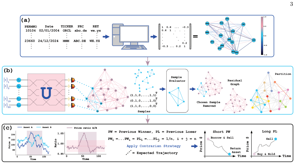
The load-bearing object is the GBS device used as a dense-subgraph sampler. A symmetric non-negative adjacency matrix is encoded into squeezing parameters and an interferometer unitary via Takagi-Autonne decomposition; the probability of a detected photon pattern is proportional to the hafnian of the corresponding submatrix, which counts perfect matchings and therefore favors dense subgraphs. GBS Roots and GBS Boost iterate by feeding the residual graph back into the sampler, selecting samples by weighted density (the normalized sum of intra-cluster edge weights), and merging or extracting them greedily into a partition. Displaced GBS adds mode-specific coherent displacements that restore th
Load-bearing premise
The benchmark comparison rests on the permutation-calibrated eigenvalue-spacing rule that fixes the cluster count K for Spectral and SPONGE; if that rule is miscalibrated for the chosen universes, the classical methods are handicapped and the quantum methods' advantage—which comes partly from not needing a preset K—is inflated.
What would settle it
Repeat the 100-stock 2020 backtest with K for the classical algorithms set by an independent standard criterion (for example, explained-variance cutoff or silhouette score) instead of the paper's eigenvalue-spacing rule. If Spectral or SPONGE then matches or exceeds GBS Roots' total return, the claimed quantum edge is an artifact of the K estimator. A second check: force GBS Roots to terminate at the same K chosen for the classical methods and see whether the advantage persists.
If this is right
- In the lossless 100-stock 2020 backtest, GBS Roots and GBS Boost rank above SPONGE and Spectral on total return, and GBS Roots' return edge over SPONGE is statistically significant at the 5% level while its Sharpe ratio is statistically indistinguishable at lower variance.
- Coherent displacement flattens the performance decay under photon loss, keeping GBS methods competitive with classical benchmarks at loss rates where uncompensated GBS falls to a random clustering baseline.
- The quantum edge concentrates in high-volatility regimes: quantum Sharpe ratios track the VIX, with the largest gains in 2008 and 2020 and underperformance in the low-volatility 2017 regime.
- Larger stock universes favor the quantum methods: return distributions develop a heavier right tail beyond roughly N=30, while classical methods show tighter but lower-upside return profiles.
- Maximizing graph density or weighted density does not by itself maximize economic return—SPONGE holds the highest weighted density yet trails the quantum methods—so the authors' partition objective is a necessary but incomplete bridge to PnL.
Where Pith is reading between the lines
- The comparison is asymmetric by design—classical methods receive a data-driven K while GBS methods terminate organically; a direct control that feeds each classical method the same number of clusters the GBS partition produces (or forces GBS to stop at the classical K) would isolate how much of the reported edge is the freedom not to preselect K.
- Because the simulations cover only 10–20% of the S&P 500 and assume zero transaction costs and price impact, the economic magnitudes are upper bounds; a full-universe test with realistic costs could shrink the gap even if the ranking survives.
- The authors' observation that photon loss acts as an implicit regulariser suggests a purely classical analogue: injecting controlled noise into the adjacency matrix before spectral clustering might reproduce some of GBS's diversification benefit, which would indicate the edge is stochasticity rather than quantum hardware.
- Replacing the weighted-density selection rule with an Ornstein-Uhlenbeck mean-reversion speed estimate (which the paper identifies as future work) could change the ranking of methods; if it helps classical clustering more than GBS, part of the quantum advantage is tied to the current selection metric.
Editorial analysis
A structured set of objections, weighed in public.
Referee Report
Summary. The paper applies Gaussian Boson Sampling (GBS) to asset clustering for statistical arbitrage. It maps S&P 500 residual-return correlation matrices into non-negative adjacency matrices, adapts GBS Boost, and introduces a novel GBS Roots clustering algorithm, benchmarking them against classical Spectral, SPONGE, and a classical GBS proxy (QIC-GBS). The main empirical claims are (i) in a lossless 100-stock universe over 2020, GBS-derived clustering yields superior total returns relative to classical Spectral and SPONGE; (ii) under photon loss, displacement compensation restores economic competitiveness; and (iii) quantum methods perform best in volatile regimes. The analysis uses simulated GBS via Strawberry Fields, with a rolling 3-day rebalancing StatArb strategy.
Significance. If substantiated, this would be a notable empirical demonstration that a photonic GBS heuristic can add economic value in a concrete quantitative-finance task, going beyond abstract graph benchmarks. The paper has real strengths: it provides a detailed strategy specification, uses public data and an open simulation framework, tests multiple market regimes, and analyzes photon-loss effects with a proposed displacement compensation. These features make the claims reproducible and falsifiable. However, the central economic claim currently rests on a small number of simulation runs, a single large-universe sample year, and a classical baseline whose cluster-count input is set by a custom, unvalidated estimator. The reported statistical support is a single uncorrected t-test. These are load-bearing weaknesses, but they are addressable within the manuscript's scope.
major comments (5)
- [Section IV.A; Appendix B, Eq. (B6)] The classical baselines require a target cluster count K, which is supplied by the permutation-calibrated eigenvalue-spacing estimator of Appendix B. This estimator is load-bearing: if it systematically under- or over-estimates K on the 2020 correlation matrices, Spectral and SPONGE are handicapped and the reported quantum outperformance may be an artifact. No synthetic test shows that Eq. (B6) recovers a known number of clusters, and no sensitivity analysis reports classical performance as a function of K. The defense in Appendix A that the market-informed 'oracle' strengthens the quantum result presupposes that the oracle is accurate. Please add a grid search over K for the classical methods, a synthetic cluster-recovery validation, and a plot of classical total return versus K.
- [Table I and Section IV.A] The statistical support for the headline claim is one two-tailed Welch t-test comparing terminal returns of GBS Roots vs SPONGE (p = 0.023), uncorrected for the multiple pairwise comparisons and metrics examined. This p-value is marginal, and it does not cover GBS Boost, whose outperformance over SPONGE (0.239 vs 0.214) is not tested. The run counts also differ: ~20 quantum runs vs ~100 classical runs. Please report all pairwise comparisons with a multiple-testing correction (or a pre-specified primary comparison), bootstrap confidence intervals for the differences, and, where possible, matched-seed paired tests.
- [Section IV.B, Figure 4; Appendices G-H] The loss-displacement claims are stated with qualitative terms such as 'frequently outperform' and '85% of cases' (loss ≤ 40%), but no run-level statistical tests or confidence intervals are provided for these statements. In addition, the displacement compensation procedure is asserted to preserve 'the relative weights of the encoded residual correlations' (Appendix G), yet this invariance is not proven or numerically verified. Without such validation, the recovery at high loss could be a coincidental consequence of the specific displacement parametrization. Please provide formal conditions or numerical checks for the invariance claim, and report error bars and tests for the loss-rate comparisons.
- [Section V and Appendix A, Eq. (A3)] All return figures are gross of transaction costs and price impact, as acknowledged in Section V. Given the strategy rebalances every 3 days with a p=0 signal threshold and holds a 100-stock universe, turnover is potentially large; the ranking in Table I may not survive realistic trading costs. Please report average turnover per algorithm, break-even transaction costs, and a sensitivity analysis under a range of cost/impact assumptions. Without this, the 'economic competitiveness' claim is not fully supported.
- [Section IV.A vs IV.C and Appendix J] The large-universe lossless claim is based on a single year (2020, N=100). The other regimes in Section IV.C use N=50, and Appendix J shows non-monotonic performance as the universe scales from 12 to 50 stocks. The abstract's broader statement about 'large stock universes' and 'distinct macroeconomic regimes' therefore rests on one large-universe sample. Please either extend the large-universe lossless analysis to additional years or explicitly restrict the claim to the 2020 sample, with appropriate caveats.
minor comments (4)
- [Appendix G, Eq. (G5)] With the ansatz p_epsilon = Omega(1/N), the bound should be delta_max = exp(-F N log N * p_epsilon) = N^{-F c} for some constant c, not N^{-F}. The constant matters for the stated 'F >= 1' sufficiency threshold; please make the constant explicit or rephrase.
- [Section III] The sentence 'Applying it purely as a structural heuristic is insufficient' appears twice in quick succession; one copy should be removed.
- [Table II] The cluster value V is reported for 'the best partition (by total return)'. Selecting the best run by the outcome variable means V reflects an in-sample selected run, not the algorithm's typical partition; please clarify or report the average/median V across runs.
- [Figure 4] Classical benchmarks are shown as horizontal lines without uncertainty bands, while quantum methods have shaded bands. Adding classical confidence intervals would make the visual comparisons more balanced.
Circularity Check
No significant circularity: the central claim is an out-of-sample backtest, not a derivation; the flagged K-calibration and p_epsilon ansatz are benchmark-fairness/rigor concerns, not definitional reductions.
full rationale
The load-bearing assertion is an empirical backtest comparison, not a derivation whose conclusion is encoded in its inputs. Appendix A defines the StatArb pipeline (residual correlations over a 5-day lookback, clustering, then a 3-day forward holding period), and Equation (A3) computes returns from subsequent price movements; no quantum or classical clustering parameter is fitted to those forward returns. The GBS algorithms' only role is to propose partitions, and the paper explicitly shows that the clustering objective and economic performance decouple: SPONGE achieves the highest weighted density but trails the quantum methods in total return (Section IV.A). Thus the reported 'superior alpha' is not equivalent by construction to the value function in Eq. (1). The two candidate concerns do not amount to circularity. First, the classical K estimator in Appendix B is calibrated on the same window data, but this is a benchmark-fairness issue: the quantum results are not derived from K, and the paper itself flags the finite-sample breakdown of the TW asymptotics and resorts to permutation calibration. Second, Appendix G's sample-complexity bound explicitly invokes 'the ansatz p_epsilon = Omega(1/N)', an unverified assumption that makes the bound conditional; a missing or assumed premise is a rigor gap rather than a self-referential reduction. Self-citations to Refs. [34], [37], and [53] involve co-author Cucuringu, but SPONGE and Spectral are published, externally falsifiable benchmarks, not an internal uniqueness theorem used to force the conclusion. The paper's own stated limitations (zero transaction costs, restricted universe, finite-sample calibration) reduce external validity but do not make the derivation circular.
Axiom & Free-Parameter Ledger
free parameters (5)
- Mean photon number \bar{n} =
sqrt(dim(A))
- GBS sample budget H =
F N log N, F ∈ {0.6,0.7,1.0} (and 5NlogN in Appendix J)
- K-selection calibration (τ, B, α) =
τ = q_{1−α} N^{−2/3}, B=1000, α=0.05
- Trading hyperparameters =
60-day beta window, 5-day correlation lookback, l=3-day holding, q=0.02 stop-win, p=0
- Displacement amplitudes α_i (DGBS) =
chosen to satisfy \bar{n}_tot^{(c)} = η Σ sinh² r_i + Σ |α_i|²
axioms (6)
- standard math Marchenko-Pastur theorem and BBP phase transition describe the eigenvalue spectrum of residual-return correlation matrices.
- domain assumption Single-factor beta residualization removes the market mode, leaving residual returns that are approximately uncorrelated under the null.
- domain assumption GBS sampling preferentially draws dense subgraphs, and this bias persists for the thresholded non-negative adjacency matrix max(0,C−I).
- domain assumption Photon loss can be modeled by uniformly rescaling the adjacency matrix A→ηA (small-squeezing approximation).
- ad hoc to paper The ε-optimal hit rate satisfies p_ε = Ω(1/N) for financial correlation graphs.
- ad hoc to paper Displacement compensation preserves the relative weights of encoded residual correlations.
read the original abstract
Gaussian Boson Sampling (GBS) provides a native photonic quantum heuristic for sampling dense subgraphs from adjacency matrices, offering a scalable physical approach to combinatorial graph search problems. Simultaneously, correlation matrix clustering algorithms, such as Spectral and SPONGE, have established robust benchmarks for identifying co-moving assets from correlation matrices in statistical arbitrage (StatArb) strategies. In this work, we map S&P 500 residual correlation data into GBS-compatible adjacency matrices. We benchmark those classical clustering algorithms against two quantum clustering algorithms, GBS Boost and our novel GBS Roots, to construct dynamic, market-neutral portfolios over a rolling one-year window. Simulations across distinct macroeconomic regimes reveal that quantum clustering generates superior alpha within large stock universes during periods of high volatility, effectively isolating structural market idiosyncrasies. Crucially, this economic advantage persists under simulated low-loss conditions and extends into high-loss regimes via the application of coherent displacement to compensate for photon loss. Our findings underscore the efficacy of GBS-derived graph clustering in constructing robust StatArb portfolios, establishing a quantum foundation for broader quantitative finance applications.
Figures


Reference graph
Works this paper leans on
-
[1]
Stamatopoulos, D
N. Stamatopoulos, D. J. Egger, Y. Sun, C. Zoufal, R. Iten, N. Shen, and S. Woerner, Quantum4, 291 (2020)
2020
-
[2]
Slate, E
N. Slate, E. Matwiejew, S. Marsh, and J. B. Wang, Quan- tum5, 513 (2021)
2021
-
[3]
Y. J. Chang, W.-T. Wang, Y.-Y. Wang, C.-Y. Liu, K.-C. Chen, and C.-R. Chang, arXiv preprint arXiv:2507.03963 (2025)
arXiv 2025
-
[4]
Or´ us, S
R. Or´ us, S. Mugel, and E. Lizaso, Reviews in Physics4, 100028 (2019)
2019
-
[5]
Rosenberg, P
G. Rosenberg, P. Haghnegahdar, P. Goddard, P. Carr, K. Wu, and M. L. De Prado, inProceedings of the 8th workshop on high performance computational finance (2015), pp. 1–7
2015
-
[6]
Aaronson and A
S. Aaronson and A. Arkhipov, inProceedings of the forty- third annual ACM symposium on Theory of computing (2011), pp. 333–342
2011
-
[7]
C. S. Hamilton, R. Kruse, L. Sansoni, S. Barkhofen, C. Silberhorn, and I. Jex, inCLEO: QELS Fundamental Science(Optica Publishing Group, 2017), pp. FTu1F–2
2017
-
[8]
H.-S. Zhong, H. Wang, Y.-H. Deng, M.-C. Chen, L.-C. Peng, et al., Science370, 1460 (2020), https://www.science.org/doi/pdf/10.1126/science.abe8770, URLhttps://www.science.org/doi/abs/10. 1126/science.abe8770
-
[9]
Zhong, Y.-H
H.-S. Zhong, Y.-H. Deng, J. Qin, H. Wang, M.-C. Chen, et al., Phys. Rev. Lett.127, 180502 (2021), URLhttps://link.aps.org/doi/10.1103/ PhysRevLett.127.180502
2021
-
[10]
L. S. Madsen, F. Laudenbach, M. Falamarzi. Askarani, F. Rortais, T. Vincent, et al., Nature606, 75 (2022), ISSN 1476-4687
2022
-
[11]
Deng, Y.-C
Y.-H. Deng, Y.-C. Gu, H.-L. Liu, S.-Q. Gong, H. Su, et al., Phys. Rev. Lett.131, 150601 (2023), URLhttps://link.aps.org/doi/10.1103/ PhysRevLett.131.150601
2023
-
[12]
H.-L. Liu, H. Su, Y.-H. Deng, S.-Q. Gong, Y.-C. Gu, H.- Y. Tang, M.-H. Jia, Q. Wei, Y.-K. Song, D.-Z. Wang, et al., Nature pp. 1–6 (2026)
2026
-
[13]
C. Oh, K. Noh, B. Fefferman, and L. Jiang, Physical Review Letters128, 190501 (2022)
2022
-
[14]
C. Oh, M. Liu, Y. Alexeev, B. Fefferman, and L. Jiang, Nature Physics20, 1461 (2024)
2024
-
[15]
M. Liu, C. Oh, J. Liu, L. Jiang, and Y. Alexeev, Physical Review A108, 052604 (2023)
2023
-
[16]
Zhang, S
Y. Zhang, S. Zhou, X. Wang, Z. Wang, Z. Yang, R. Yang, 11 Y. Xue, and T. Li, Nature Communications16, 9335 (2025)
2025
-
[17]
S.-Q. Gong, M.-C. Chen, H.-L. Liu, H. Su, Y.-C. Gu, H.- Y. Tang, M.-H. Jia, Y.-H. Deng, Q. Wei, H. Wang, et al., arXiv preprint arXiv:2506.19707 (2025)
Pith/arXiv arXiv 2025
-
[18]
H. Zhu, W. Luo, R. Yan, C. Ren, J. Guo, Z. Zhao, H. Ma, T. Chen, F. Gao, L. C. Kwek, et al., Research (2025)
2025
-
[19]
D. Montesinos, G. L. Giorgi, and R. Zambrini, arXiv preprint arXiv:2606.15230 (2026)
arXiv 2026
-
[20]
J. Huh, G. G. Guerreschi, B. Peropadre, J. R. McClean, and A. Aspuru-Guzik, Nature Photonics9, 615 (2015)
2015
-
[21]
Banchi, M
L. Banchi, M. Fingerhuth, T. Babej, C. Ing, and J. M. Arrazola, Science advances6, eaax1950 (2020)
2020
-
[22]
S. He, B. Ai, P. Gao, H. Liu, J.-J. He, K.-M. Hu, Y.-Z. Zhu, and J. Wu, Chip p. 100181 (2025)
2025
-
[23]
Yu, Z.-P
S. Yu, Z.-P. Zhong, Y. Fang, R. B. Patel, Q.-P. Li, W. Liu, Z. Li, L. Xu, S. Sagona-Stophel, E. Mer, et al., Nature Computational Science3, 839 (2023)
2023
-
[24]
S. Yu, J. Sun, Z. Li, E. Mer, Y. K. Alwehaibi, O. Scholin, G. J. Machado, K.-C. Chen, A. Zhang, R. B. Patel, et al. (2025), arXiv:2507.08157, URLhttps://arxiv.org/ abs/2507.08157
Pith/arXiv arXiv 2025
-
[25]
H.-Y. Huang, S. Choi, J. R. McClean, and J. Preskill, Phys. Rev. X16, 030501 (2026), URLhttps://link. aps.org/doi/10.1103/tn89-g1xz
-
[26]
Br´ adler, P.-L
K. Br´ adler, P.-L. Dallaire-Demers, P. Rebentrost, D. Su, and C. Weedbrook, Physical Review A98, 032310 (2018)
2018
-
[27]
J. M. Arrazola and T. R. Bromley, Physical review letters 121, 030503 (2018)
2018
-
[28]
Schuld, K
M. Schuld, K. Br´ adler, R. Israel, D. Su, and B. Gupt, Physical Review A101, 032314 (2020)
2020
-
[29]
G. E. Uhlenbeck and L. S. Ornstein, Physical review36, 823 (1930)
1930
-
[30]
Deng, S.-Q
Y.-H. Deng, S.-Q. Gong, Y.-C. Gu, Z.-J. Zhang, H.-L. Liu, H. Su, H.-Y. Tang, J.-M. Xu, M.-H. Jia, M.-C. Chen, et al., Physical Review Letters130, 190601 (2023)
2023
-
[31]
K. Br´ adler, S. Friedland, J. Izaac, N. Killoran, and D. Su, arXiv preprint arXiv:1810.10644 (2018)
Pith/arXiv arXiv 2018
-
[32]
J. Epequin, P. Bendotti, and J. Mikael, arXiv preprint arXiv:2601.20263 (2026)
arXiv 2026
-
[33]
Bonaldi, M
N. Bonaldi, M. Rossi, D. Mattioli, M. Grapulin, B. S. Fern´ andez, D. Caputo, M. Magagnini, A. Osti, and F. Veronese, Quantum Machine Intelligence6, 65 (2024)
2024
-
[34]
Q. Jin, M. Cucuringu, and ´A. Cartea, inProceedings of the Fourth ACM International Conference on AI in Fi- nance(2023), pp. 557–564. [35]Wharton research data services,https://wrds-www. wharton.upenn.edu/, accessed: 2025-05
2023
-
[36]
A. Ng, M. Jordan, and Y. Weiss, Advances in neural information processing systems14(2001)
2001
-
[37]
Cucuringu, P
M. Cucuringu, P. Davies, A. Glielmo, and H. Tyagi, in The 22nd International Conference on Artificial Intelli- gence and Statistics(PMLR, 2019), pp. 1088–1098
2019
-
[38]
C. Oh, B. Fefferman, L. Jiang, and N. Quesada, PRX Quantum5, 020341 (2024), URLhttps://link.aps. org/doi/10.1103/PRXQuantum.5.020341
-
[39]
Bansal, A
N. Bansal, A. Blum, and S. Chawla, Machine learning 56, 89 (2004)
2004
-
[40]
Treleaven, M
P. Treleaven, M. Galas, and V. Lalchand, Communica- tions of the ACM56, 76 (2013)
2013
-
[41]
R. J. Elliott, J. Van Der Hoek*, and W. P. Malcolm, Quantitative Finance5, 271 (2005)
2005
-
[42]
Avellaneda and J.-H
M. Avellaneda and J.-H. Lee, Quantitative Finance10, 761 (2010)
2010
-
[43]
Krauss, Journal of Economic Surveys31, 513 (2017)
C. Krauss, Journal of Economic Surveys31, 513 (2017)
2017
-
[44]
S. Yu, J. Sun, K.-C. Chen, Z.-H. Yang, Z. Li, E. Mer, Y. K. Alwehaibi, S. H. Winston, D. M. Lopena, Z.-C. Zhang, et al. (2026), arXiv:2602.06544, URLhttps:// arxiv.org/abs/2602.06544
arXiv 2026
-
[45]
D. J. Egger, J. Mareˇ cek, and S. Woerner, Quantum5, 479 (2021)
2021
-
[46]
Y. Yu, X.-B. Wang, N. Shannon, and R. Joynt, arXiv preprint arXiv:2503.20048 (2025)
Pith/arXiv arXiv 2025
-
[47]
Shakiba, Knowledge and Information Systems pp
A. Shakiba, Knowledge and Information Systems pp. 1– 20 (2025)
2025
-
[48]
Davies, B
S. Davies, B. Moseley, and H. Newman, inInternational Conference on Machine Learning(PMLR, 2023), pp. 7205–7230
2023
-
[49]
A. Macaluso, S. M. Venkatesh, D. Arenas, M. Klusch, and A. Dengel, arXiv preprint arXiv:2509.03561 (2025)
arXiv 2025
-
[50]
S. M. Venkatesh, A. Macaluso, and M. Klusch, in International Conference on Computational Science (Springer, 2023), pp. 138–152
2023
-
[51]
Willsch, D
M. Willsch, D. Willsch, F. Jin, H. De Raedt, and K. Michielsen, Quantum Information Processing19, 197 (2020)
2020
-
[52]
Bapst, L
V. Bapst, L. Foini, F. Krzakala, G. Semerjian, and F. Zamponi, Physics Reports523, 127 (2013)
2013
-
[53]
Cucuringu, A
M. Cucuringu, A. V. Singh, D. Sulem, and H. Tyagi, Journal of Machine Learning Research22, 1 (2021)
2021
-
[54]
Thekkadath, S
G. Thekkadath, S. Sempere-Llagostera, B. Bell, R. Pa- tel, M. Kim, and I. Walmsley, PRX Quantum3, 020336 (2022), ISSN 2691-3399
2022
-
[55]
J. Liu, F. Wilde, A. A. Mele, X. Jin, L. Jiang, and J. Eis- ert, Physical Review A111, 052441 (2025)
2025
-
[56]
R. A. Maller, G. M¨ uller, and A. Szimayer, Handbook of financial time series pp. 421–437 (2009)
2009
-
[57]
E. Mer, Z. Li, S. Yu, I. A. Walmsley, and R. B. Patel (2026), arXiv:2605.27522, URLhttps://arxiv.org/ abs/2605.27522
Pith/arXiv arXiv 2026
-
[58]
D. M. Lopena and D. Buguks,https://doi.org/10. 5281/zenodo.18890167(2026)
2026
-
[59]
I. M. Johnstone, The Annals of statistics29, 295 (2001)
2001
-
[60]
Baik and J
J. Baik and J. W. Silverstein, Journal of multivariate analysis97, 1382 (2006)
2006
-
[61]
J. Baik, G. Ben Arous, and S. P´ ech´ e, The Annals of Probability (2005)
2005
-
[62]
Dvoretzky, J
A. Dvoretzky, J. Kiefer, and J. Wolfowitz, The Annals of Mathematical Statistics pp. 642–669 (1956)
1956
-
[63]
Massart, The annals of Probability pp
P. Massart, The annals of Probability pp. 1269–1283 (1990)
1990
-
[64]
Kruse, C
R. Kruse, C. S. Hamilton, L. Sansoni, S. Barkhofen, C. Silberhorn, and I. Jex, Physical Review A100, 032326 (2019)
2019
-
[65]
Jerrum, A
M. Jerrum, A. Sinclair, and E. Vigoda, Journal of the ACM (JACM)51, 671 (2004)
2004
-
[66]
A. Uvarov and D. Vinichenko, Phys. Rev. A109, 042415 (2024), URLhttps://link.aps.org/doi/ 10.1103/PhysRevA.109.042415
-
[67]
K. Anand, Z. Chen, M. Cryan, G. Freifeld, L. A. Goldberg, H. Guo, and X. Zhang,Simulating gaus- sian boson sampling on graphs in polynomial time (2025), 2511.16558, URLhttps://arxiv.org/abs/ 2511.16558
Pith/arXiv arXiv 2025
-
[68]
Yang and X.-B
T.-Y. Yang and X.-B. Wang, Scientific Reports14, 7680 (2024). 12
2024
-
[69]
Roughgarden,Algorithms Illuminated (Part 2) Graph Algorithms and Data Structures (Volume 2)(Soundlikey- ourself Publishing, LLC, 2018)
T. Roughgarden,Algorithms Illuminated (Part 2) Graph Algorithms and Data Structures (Volume 2)(Soundlikey- ourself Publishing, LLC, 2018)
2018
-
[70]
Aaghabali, S
M. Aaghabali, S. Akbari, S. Friedland, K. Markstr¨ om, and Z. Tajfirouz, European Journal of Combinatorics45, 132 (2015)
2015
-
[71]
T. R. Bromley, J. M. Arrazola, S. Jahangiri, J. Izaac, N. Quesada, A. D. Gran, M. Schuld, J. Swinarton, Z. Za- baneh, and N. Killoran, Quantum Science and Technol- ogy5, 034010 (2020)
2020
-
[72]
Garc ´ ıa-Patr´ on, J
R. Garc ´ ıa-Patr´ on, J. J. Renema, and V. Shchesnovich, Quantum3, 169 (2019)
2019
-
[73]
Oszmaniec and D
M. Oszmaniec and D. J. Brod, New Journal of Physics 20, 092002 (2018)
2018
-
[74]
Y. Zhao, X.-Y. Xu, C.-F. Li, and G.-C. Guo, arXiv preprint arXiv:2512.00753 (2025)
Pith/arXiv arXiv 2025
-
[75]
Weedbrook, S
C. Weedbrook, S. Pirandola, R. Garc ´ ıa-Patr´ on, N. J. Cerf, T. C. Ralph, J. H. Shapiro, and S. Lloyd, Reviews of Modern Physics84, 621 (2012)
2012
-
[76]
S. L. Braunstein, Physical Review A—Atomic, Molecu- lar, and Optical Physics71, 055801 (2005)
2005
-
[77]
Quesada and J
N. Quesada and J. M. Arrazola, Physical Review Re- search2, 023005 (2020)
2020
-
[78]
Sempere-Llagostera, R
S. Sempere-Llagostera, R. Patel, I. Walmsley, and W. Kolthammer, Physical Review X12, 031045 (2022)
2022
-
[79]
L. G. Valiant, Commun. ACM27, 1134–1142 (1984), ISSN 0001-0782, URLhttps://doi.org/10.1145/ 1968.1972
arXiv 1984
-
[80]
N. Killoran, J. Izaac, N. Quesada, V. Bergholm, M. Amy, and C. Weedbrook, Quantum3, 129 (2019), 1804.03159
Pith/arXiv arXiv 2019
-
[81]
Quesada, J
N. Quesada, J. M. Arrazola, and N. Killoran, Physical Review A98, 062322 (2018)
2018
discussion (0)
Sign in with ORCID, Apple, or X to comment. Anyone can read and Pith papers without signing in.