REVIEW 3 major objections 5 minor 119 references
A two-branch graph neural network, trained across randomly sampled systematic shifts, estimates the Higgs signal strength μ and its 68% confidence interval with empirical coverage of 66–68% in pseudo-experiments.
Reviewed by Pith at T0; open to challenge. T0 means a machine referee read the full paper against a public rubric. the ladder, T0–T4 →
SAGE, a dual-branch GNN trained under nuisance fluctuations, estimates the Higgs signal strength with near-nominal coverage (0.662-0.683) but wider intervals than the top FAIR-HUC leaderboard methods.
T0 review reviewed 2026-08-05 challenge →
load-bearing objection A solid, reproducible nuisance-aware ML inference pipeline whose main accuracy claim is undermined by a consistent positive bias in the paper's own fixed-µ tests and a training-weight sensitivity that the authors disclose but do not resolve. the 3 major comments →
Higgs Signal Strength Estimation with Machine Learning under Systematic Uncertainties
The pith
A machine-rendered reading of the paper's core claim, the machinery that carries it, and where it could break.
The reading
Core claim
The paper claims that a machine-learning classifier can be made systematics-aware without giving up classical frequentist inference: split each event into a deterministic branch and an uncertainty-aware branch, train the network by injecting 100 randomly sampled nuisance configurations per epoch and averaging the classification loss over the perturbed replicas, then histogram the signal-class output into adaptively binned yields and build a Poisson surrogate likelihood whose six nuisance parameters are profiled numerically. On simulated proton-proton H→ττ events with three calibration-type and three normalization-type uncertainties, this pipeline returns maximum-likelihood estimates of the s
What carries the argument
The central object is a dual-branch graph neural network: a deterministic GNN passes only nuisance-independent node, edge, and global features, while an uncertainty-aware GNN—using gated attention-based message passing—handles features shifted by the three calibration-type nuisances. Training draws 100 nuisance vectors per epoch and averages the cross-entropy loss over the perturbed replicas, decorrelating the classifier output from nuisance shifts. Downstream, binned signal-class probabilities feed region-wise trilinear interpolation tables over the three calibration parameters; these tables enter a Poisson likelihood with Gaussian priors on the nuisance parameters, and numerical minimizati
Load-bearing premise
The headline interval widths depend on training with uniform per-event weights even though the Higgs signal is heavily oversampled relative to its physical yield; if one instead trains with weights that reflect the real event composition, the confidence intervals become systematically wider, so the stated precision rests on that training choice.
What would settle it
Retrain the classifier with per-event weights set to physical yields (cross-section times luminosity) instead of uniform weights, rerun the 50,000 pseudo-experiments, and compare the average 68.27% interval width with 0.634; the appendix's class-frequency retraining already shows the widths widen, so this calculation would settle whether the headline precision is tied to the training weighting.
If this is right
- If the central claim holds, LHC-style measurements can use high-dimensional GNN classifiers as the front end of a profile-likelihood fit, with nuisance parameters constrained by classifier-enriched control regions.
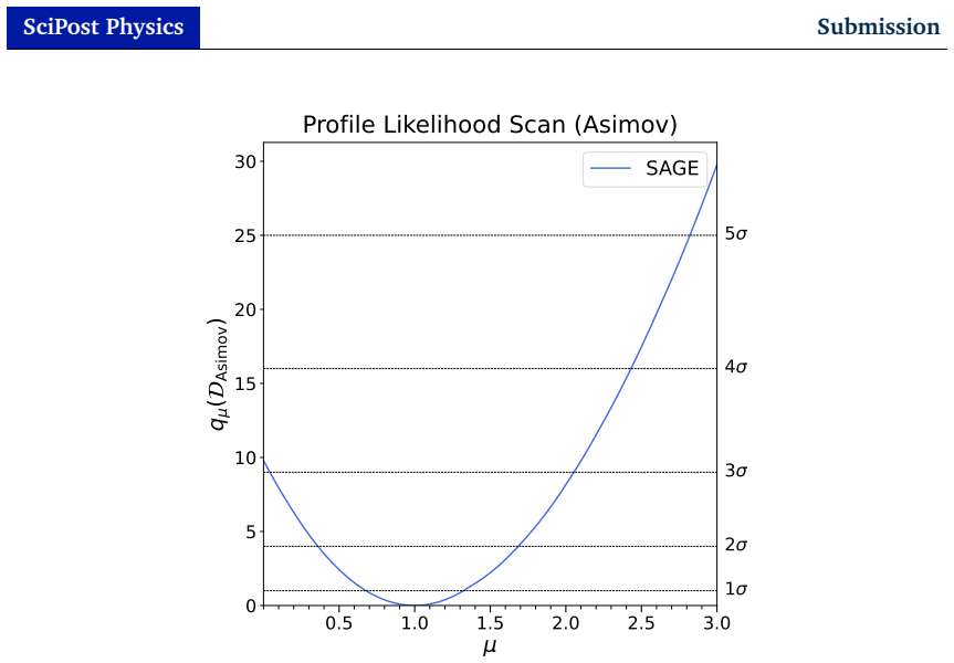
- The Asimov fit visibly constrains the calibration nuisances—especially the tau energy scale—and the tt and diboson normalizations, so the framework returns both μ and a nuisance-parameter hierarchy in one pass.
- Training cost is dominated by the 100-fold replica augmentation, but a single pseudo-experiment fit takes minutes on a CPU and about two minutes on a GPU, making large coverage studies practical.
- The dense 17×17×41 interpolation grid is the scaling bottleneck: the network itself is claimed to be largely insensitive to the number of nuisance parameters, but constructing the table becomes increasingly challenging as that number grows.
- The method is presented as directly applicable to precision measurements at the LHC and readily extendable to final states with higher object multiplicities, where graph representations exploit multi-object correlations.
Where Pith is reading between the lines
- The appendix's class-frequency retraining leaves implicit that the coverage is stable under reweighting while the interval widths are not; a yield-weighted retraining would likely give the honest precision for real data, with the headline width of 0.634 potentially optimistic.
- Because the classifier is trained to ignore nuisance shifts rather than to output a likelihood itself, the approach remains a decorrelation strategy; pairing the nuisance-averaged loss with an inference-aware objective could sharpen sensitivity without changing the downstream morphing.
- The dense interpolation grid limits the framework to a small number of calibration nuisances; sparse grids or normalizing flows, which the paper names as future work, would determine whether the approach reaches the full six-parameter systematic space.
- The quoted comparison with leaderboard methods is conditional: the paper notes the protocols are not identical, so a like-for-like re-evaluation is needed before the 'moderately wider intervals' statement becomes a ranking.
Editorial analysis
A structured set of objections, weighed in public.
Referee Report
Summary. The paper presents SAGE, a dual-branch graph neural network for estimating the Higgs boson signal strength mu in the presence of systematic uncertainties. A deterministic GNN and an uncertainty-aware GNN process disjoint feature sets, and training averages a four-class cross-entropy loss over 100 nuisance-parameter replicas per event. The classifier output is binned in one inclusive and three control regions; interpolation tables over calibration nuisance parameters provide expected per-bin yields, and a Poisson profile likelihood with Gaussian nuisance priors is used to extract mu and 68.27% confidence intervals. Validation uses an Asimov study, 9000 fixed-mu pseudo-experiments, and 50,000 pseudo-experiments with mu drawn uniformly from [0,3]. The central claims are that the method gives accurate maximum-likelihood estimates of mu, coverage close to nominal (0.662-0.683 fixed, 0.6697 global), and competitive interval widths (average 0.6342).
Significance. If the statistical claims hold, the paper is a useful contribution: it couples a modern graph-based representation with systematics-aware training and a tractable profile-likelihood pipeline, and it provides a publicly available implementation. The validation scale is substantial (59,000 pseudo-experiments), the architecture is described in detail, and the appendix already contains a meaningful robustness check on training class weights. However, the paper's own numbers reveal a systematic bias in the point estimates and a statistically significant global under-coverage, and the headline interval widths depend on a training-weighting choice that the authors themselves state is neither luminosity-scaled nor class-balanced. These issues do not invalidate the general framework, but they must be diagnosed, quantified, and reflected in the claims before the paper can be accepted.
major comments (3)
- [Sec. 5.2, Fig. 8; Sec. 5.3; Abstract; Sec. 6] The fixed-mu pseudo-experiments show a systematic positive bias in the MLEs of mu. The mean fitted values in Fig. 8 are 0.392, 0.664, 0.973, 1.265, 1.535, 1.842, 2.152, 2.449, 2.712 for true values 0.3, 0.6, 0.9, 1.2, 1.5, 1.8, 2.1, 2.4, 2.7, i.e. offsets of roughly +0.09, +0.06, +0.07, +0.07, +0.04, +0.04, +0.05, +0.05, +0.01. With 1000 toys per point and a per-toy RMS of order 0.3 (inferred from the quoted 68% interval widths), the standard error of each mean is about 0.01, so most of these offsets are several standard deviations from zero. This directly contradicts Sec. 5.3's statement that the scatter shows 'no significant bias or outliers' and is inconsistent with the abstract's and Sec. 6's claim of 'accurate maximum likelihood estimates'. The authors should quantify the bias, diagnose its origin (boundary truncation at mu=0, quadratic refinement near the minimum, or nuisance profi
- [Sec. 5.3, Fig. 11] The global coverage of the 68.3% intervals is reported as 0.6697 from 50,000 pseudo-experiments. Under the null hypothesis of nominal coverage, the binomial standard error is sqrt(0.6827*0.3173/50000) = 0.00208, so the observed value is about 6 standard deviations below 0.6827. The statement that deviations are 'small fluctuations consistent with expected sampling noise from 50000 pseudo-experiments' is therefore not supported. This is a modest but real under-coverage, and together with the average width of 0.6342 it suggests the intervals are somewhat too narrow. If the 95% intervals are also claimed to have excellent coverage, the numerical global coverage for those intervals should be reported. The authors should investigate the source (Wilks approximation, interpolation bias, or boundary effects) and discuss the magnitude honestly.
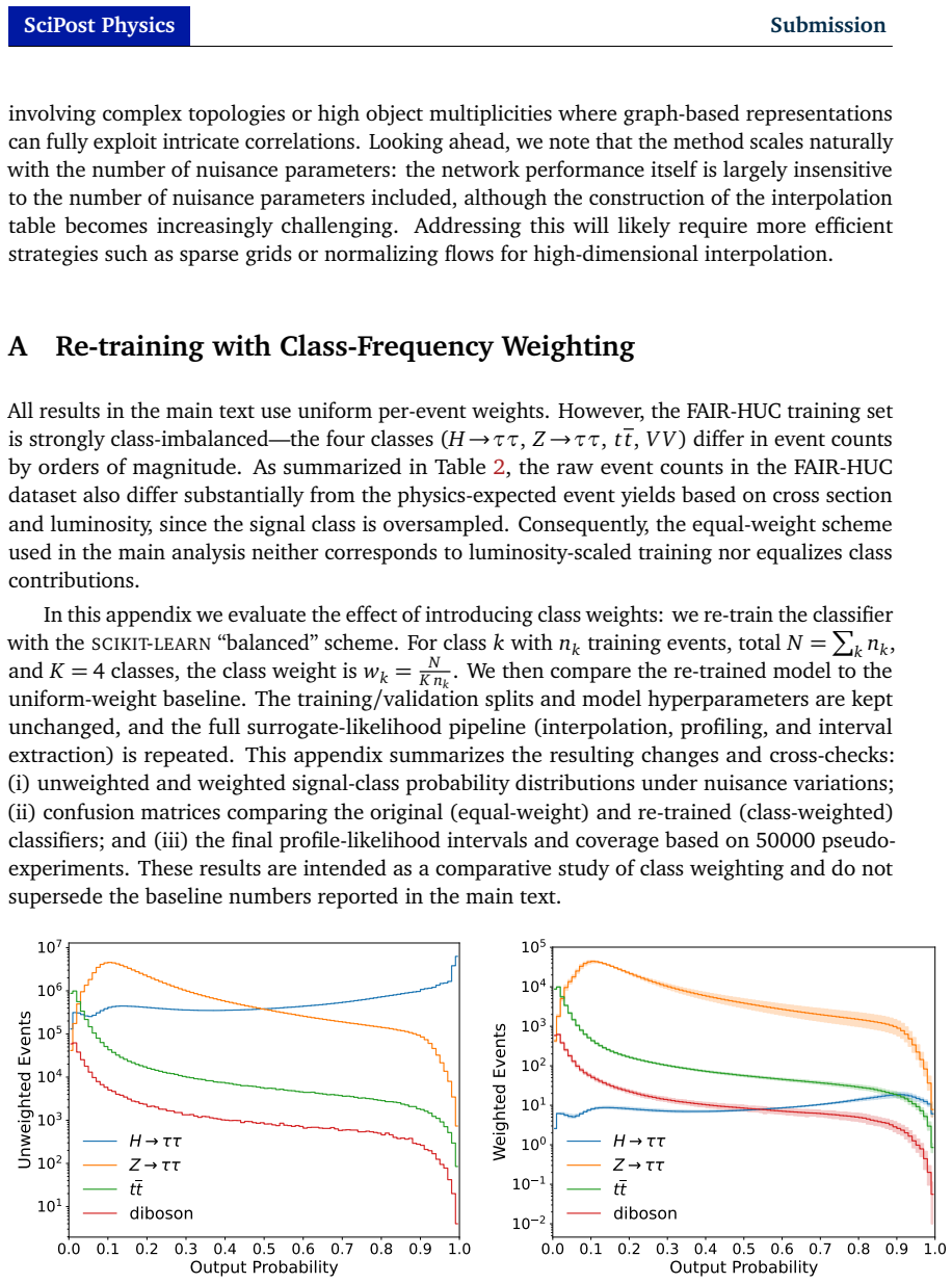
- [Sec. 3.1; Appendix A, Table 7, Fig. 14] The main analysis trains the classifier with uniform per-event weights even though the FAIR-HUC training sample is strongly class-imbalanced and the signal class is heavily oversampled relative to its physical yield (Table 2). Appendix A shows that retraining with class-frequency weights leaves coverage essentially unchanged but systematically widens the confidence intervals (Fig. 14). The authors themselves note in Appendix A that the equal-weight scheme 'neither corresponds to luminosity-scaled training nor equalizes class contributions'. Since the headline 'competitive interval widths' depend on this training choice, the paper should either justify uniform weighting as part of the analysis prescription or present the class-frequency-weighted results as the primary/conservative configuration. At minimum, the abstract and conclusions should not present the quoted widths as intrinsic pro
minor comments (5)
- [Sec. 5.3, Eq. (19)/(20)] The text says the empirical coverage is 'defined in (19)', but Eq. (19) defines the interval width and Eq. (20) defines the coverage. Please correct the cross-reference.
- [Sec. 2.3 and Sec. 4.2] The parameterization alpha_met = exp(nu_met) - 1 with nu_met ~ N(0,1) gives alpha_met median 0 but mean exp(0.5)-1 = 0.648. The phrase in Sec. 2.3 describing alpha_met as a log-normal nuisance parameter 'with mean 0' is ambiguous and should specify mean zero in log-space.
- [Sec. 4.2] The text describes the interpolation grid as a hypercube extending to +-4 sigma along each axis, but the alpha_met range [0,5] is not symmetric around the nominal value. Please clarify the corresponding nu_met grid and its relation to the stated +-4 sigma coverage.
- [Sec. 4.1] The adaptive binning criterion says each remaining bin must contain 'at least ten effective weighted events from the H->tau tau signal process and all three major backgrounds'. It is ambiguous whether this means at least ten events per process or ten total; please specify.
- [Sec. 5.3] The comparison with the FAIR Universe leaderboard results is appropriately qualified as not being like-for-like, but the word 'competitive' in the abstract and conclusions should carry the same qualification more explicitly, especially given the class-weighting dependence noted above.
Circularity Check
No significant circularity: the signal-strength extraction is a genuine profile-likelihood fit, and the closed-loop pseudo-experiment validation is a calibration check, not a circular reduction to inputs.
full rationale
The derivation of mu is not circular. The GNN is trained as a four-class classifier on FAIR-HUC simulated events; the signal-class output is binned and converted into process-wise expected-yield templates via interpolation tables over the three calibration nuisance parameters (Section 4.2). The profile likelihood of Eq. (13) treats mu as a free multiplicative factor on the signal template and profiles all six nuisance parameters. Nowhere is mu obtained by reading off a fitted parameter that already encodes the answer: the fixed-mu and randomized-mu pseudo-experiments are new Poisson realizations generated at injected mu_true, and the reported coverage/width numbers are Monte Carlo diagnostics of the profiling and interval-construction procedure, not identities forced by the construction. The Asimov result (Sec. 5.1), where mu_true=1 yields mu_hat=1, is a standard consistency check rather than an independent prediction. The only self-citation of potential note is Ref. [55], from which the four analysis-region selections are taken (Sec. 4.1); this is a methodological borrowing and is not load-bearing for the claim of accurate mu estimation. The paper's own fixed-mu results (Fig. 8: mean fitted values 0.392, 0.664, 0.973, 1.265, ... for true values 0.3, 0.6, 0.9, 1.2, ...) show a small systematic positive bias at every point, which is a correctness/calibration concern and an internal inconsistency with the text's 'no significant bias' statement in Sec. 5.3, but it is an empirical disagreement, not a circular reduction of the prediction to its inputs. The validation is self-referential in the sense that pseudo-data are generated from the same simulation and surrogate model used to build the likelihood, so the coverage study demonstrates internal statistical calibration rather than external physics accuracy; this limits the strength of the validation but does not constitute circularity in the equation/fitted-parameter sense.
Axiom & Free-Parameter Ledger
free parameters (4)
- Training class weighting scheme =
uniform weights (main); class-frequency weights (Appendix A)
- Adaptive binning minimum occupancy =
10 effective events per bin
- Control region score thresholds =
p_tt > 0.4, p_VV > 0.2; appendix p_VV > 0.9
- Interpolation grid resolution =
17 x 17 x 41 grid over ±4 sigma
axioms (4)
- domain assumption FAIR-HUC simulation truthfully represents H to tau tau events with the assumed nuisance parameterization.
- standard math Wilks' theorem applies to the profile likelihood ratio on this binned surrogate likelihood.
- domain assumption Trilinear interpolation of binned classifier-output yields over the nuisance grid is accurate for continuous nuisance values.
- domain assumption A single classifier trained without explicit nuisance input is sufficient; its residual nuisance dependence is captured by the interpolation tables.
Cite this review
Pith. "Pith review of Higgs Signal Strength Estimation with Machine Learning under Systematic Uncertainties." pith.science (2026). https://pith.science/paper/DMYZIORX
@misc{pith2026250900672,
  author       = {Pith},
  title        = {Pith review of: Higgs Signal Strength Estimation with Machine Learning under Systematic Uncertainties},
  year         = {2026},
  howpublished = {\url{https://pith.science/paper/DMYZIORX}},
  note         = {Machine review of arXiv:2509.00672}
}
abstract
We present a dedicated graph neural network (GNN)-based methodology for the extraction of the Higgs boson signal strength $\mu$, incorporating systematic uncertainties. The architecture features two branches: a deterministic GNN that processes kinematic variables unaffected by nuisance parameters, and an uncertainty-aware GNN that handles inputs modulated by systematic effects through gated attention-based message passing. Their outputs are fused to produce classification scores for signal-background discrimination. During training we sample nuisance-parameter configurations and aggregate the loss across them, promoting stability of the classifier under systematic shifts and effectively decorrelating its outputs from nuisance variations. The resulting binned classifier outputs are used to construct a Poisson likelihood, which enables profile likelihood scans over signal strength, with nuisance parameters profiled out via numerical optimization. We validate this framework on the FAIR Universe Higgs Uncertainty Challenge dataset, yielding accurate estimation of signal strength $\mu$ and its 68.27\% confidence interval, achieving competitive coverage and interval widths in large-scale pseudo-experiments. Our code "Systematics-Aware Graph Estimator" (SAGE) is publicly available.
Figures






Reference graph
Works this paper leans on
-
[1]
CMS, A. Tumasyan et al., A portrait of the Higgs boson by the CMS experiment ten years after the discovery., Nature 607 (2022) 7917, 60, arXiv:2207.00043 [hep-ex]. [Erratum: Nature 623, (2023)]
Pith/arXiv arXiv 2022
-
[2]
ATLAS, G. Aad et al., A detailed map of Higgs boson interactions by the ATLAS experiment ten years after the discovery, Nature 607 (2022) 7917, 52, arXiv:2207.00092 [hep-ex]. [Erratum: Nature 612, E24 (2022)]
Pith/arXiv arXiv 2022
-
[3]
ATLAS Collaboration, Search for non-resonant Higgs boson pair production in the bbℓνℓν final state with the ATLAS detector in pp collisions atps = 13 TeV, Phys. Lett. B 801 (2020) 135145, arXiv:1908.06765 [hep-ex]
Pith/arXiv arXiv 2020
-
[4]
ATLAS Collaboration, Search for Higgs boson decays into a Z boson and a light hadronically decaying resonance using 13 TeV pp collision data from the ATLAS detector, arXiv:2004.01678 [hep-ex]
Pith/arXiv arXiv 2004
-
[5]
CMS Collaboration, Inclusive search for highly boosted Higgs bosons decaying to bottom quark-antiquark pairs in proton-proton collisions atps = 13 TeV, JHEP 12 (2020) 085, arXiv:2006.13251 [hep-ex]
Pith/arXiv arXiv 2020
-
[6]
CMS Collaboration, Search for Higgs Boson and Observation of Z Boson through their Decay into a Charm Quark-Antiquark Pair in Boosted Topologies in Proton-Proton 31 SciPost Physics Submission Collisions at s=13 TeV, Phys. Rev. Lett.131 (2023) 4, 041801, arXiv:2211.14181 [hep-ex]
Pith/arXiv arXiv 2023
-
[7]
ATLAS Collaboration, Evidence of off-shell Higgs boson production from Z Z leptonic decay channels and constraints on its total width with the ATLAS detector, Phys.Lett.B 846 (4,
-
[8]
ATLAS Collaboration, Search for a resonance decaying into a scalar particle and a Higgs boson in the final state with two bottom quarks and two photons in proton-proton collisions at a center of mass energy of 13 TeV with the ATLAS detector, JHEP 11 (4, 2024) 047, arXiv:2404.12915 [hep-ex]
Pith/arXiv arXiv 2024
-
[9]
CMS Collaboration, Search for Higgs Boson Pair Production with One Associated Vector Boson in Proton-Proton Collisions atps = 13 TeV, JHEP 10 (4, 2024) 061, arXiv:2404.08462 [hep-ex]
Pith/arXiv arXiv 2024
-
[10]
ATLAS Collaboration, ATLAS searches for additional scalars and exotic Higgs boson decays with the LHC Run 2 dataset, arXiv:2405.04914 [hep-ex]
-
[11]
CMS Collaboration, Measurement of boosted Higgs bosons produced via vector boson fusion or gluon fusion in the H→b¯b decay mode using LHC proton-proton collision data atps = 13 TeV, JHEP 12 (7, 2024) 035, arXiv:2407.08012 [hep-ex]
Pith/arXiv arXiv 2024
-
[12]
G. Cowan, K. Cranmer, E. Gross, and O. Vitells,Asymptotic formulae for likelihood-based tests of new physics, Eur. Phys. J. C 71 (2011) 1554, arXiv:1007.1727 [physics.data-an]. [Erratum: Eur.Phys.J.C 73, 2501 (2013)]
Pith/arXiv arXiv 2011
-
[13]
L. H. C. G. ATLAS, CMS, Procedure for the LHC Higgs boson search combination in Summer 2011,
2011
-
[14]
Cranmer, Practical Statistics for the LHC, in 2011 European School of High-Energy Physics
K. Cranmer, Practical Statistics for the LHC, in 2011 European School of High-Energy Physics. 2014. arXiv:1503.07622 [physics.data-an]
Pith/arXiv arXiv 2011
-
[15]
CMS, A. Hayrapetyan et al., The CMS statistical analysis and combination tool: COMBINE, arXiv:2404.06614 [physics.data-an]
-
[16]
A. Andreassen and B. Nachman, Neural Networks for Full Phase-space Reweighting and Parameter Tuning, Phys. Rev. D101 (2020) 9, 091901, arXiv:1907.08209 [hep-ph]
Pith/arXiv arXiv 2020
-
[17]
M. Stoye, J. Brehmer, G. Louppe, J. Pavez, and K. Cranmer,Likelihood-free inference with an improved cross-entropy estimator, arXiv:1808.00973 [stat.ML]
-
[18]
J. Hollingsworth and D. Whiteson, Resonance Searches with Machine Learned Likelihood Ratios, arXiv:2002.04699 [hep-ph]
Pith/arXiv arXiv 2002
-
[19]
J. Brehmer, K. Cranmer, G. Louppe, and J. Pavez,Constraining effective field theories with machine learning, Phys. Rev. Lett.121 (2018) 111801, arXiv:1805.00013 [hep-ph]
Pith/arXiv arXiv 2018
-
[20]
J. Brehmer, K. Cranmer, G. Louppe, and J. Pavez,A guide to constraining effective field theories with machine learning, Phys. Rev. D98 (2018) 052004, arXiv:1805.00020 [hep-ph]
Pith/arXiv arXiv 2018
-
[21]
J. Brehmer, F . Kling, I. Espejo, and K. Cranmer,MadMiner: Machine learning-based inference for particle physics, Comput. Softw. Big Sci. 4 (2020) 3, arXiv:1907.10621 [hep-ph]. 32 SciPost Physics Submission
Pith/arXiv arXiv 2020
-
[22]
J. Brehmer, G. Louppe, J. Pavez, and K. Cranmer,Mining gold from implicit models to improve likelihood-free inference, Proc. Nat. Acad. Sci. 117 (2020) 5242, arXiv:1805.12244 [stat.ML]
Pith/arXiv arXiv 2020
-
[23]
K. Cranmer, J. Pavez, and G. Louppe,Approximating likelihood ratios with calibrated discriminative classifiers, arXiv:1506.02169 [stat.AP]
-
[24]
A. Andreassen, S.-C. Hsu, B. Nachman, N. Suaysom, and A. Suresh, Parameter Estimation using Neural Networks in the Presence of Detector Effects, Phys. Rev. D103 (2021) 036001, arXiv:2010.03569 [hep-ph]
Pith/arXiv arXiv 2021
-
[25]
A. Coogan, K. Karchev, and C. Weniger,Targeted Likelihood-Free Inference of Dark Matter Substructure in Strongly-Lensed Galaxies, 34th Conference on Neural Information Processing Systems (10, 2020) , arXiv:2010.07032 [astro-ph.CO]
Pith/arXiv arXiv 2020
-
[26]
F . Flesher, K. Fraser, C. Hutchison, B. Ostdiek, and M. D. Schwartz,Parameter Inference from Event Ensembles and the Top-Quark Mass, JHEP 09 (11, 2020) 058, arXiv:2011.04666 [hep-ph]
Pith/arXiv arXiv 2020
-
[27]
S. Bieringer, A. Butter, T . Heimel, S. Höche, U. Köthe, T . Plehn, and S. T . Radev, Measuring QCD Splittings with Invertible Networks, SciPost Phys. 10 (12, 2020) 126, arXiv:2012.09873 [hep-ph]
Pith/arXiv arXiv 2020
-
[28]
B. Nachman and J. Thaler, E Pluribus Unum Ex Machina: Learning from Many Collider Events at Once, Phys.Rev.D103 (1, 2021) 116013, arXiv:2101.07263 [physics.data-an]
Pith/arXiv arXiv 2021
-
[29]
S. Chatterjee, N. Frohner, L. Lechner, R. Schöfbeck, and D. Schwarz,Tree boosting for learning EFT parameters, Comput. Phys. Commun. 277 (2022) 108385, arXiv:2107.10859 [hep-ph]
Pith/arXiv arXiv 2022
-
[30]
S. Shirobokov, V . Belavin, M. Kagan, A. Ustyuzhanin, and A. G. Baydin,Black-Box Optimization with Local Generative Surrogates, arXiv:2002.04632 [cs.LG]
Pith/arXiv arXiv 2002
-
[31]
S. Mishra-Sharma and K. Cranmer, A neural simulation-based inference approach for characterizing the Galactic Centerγ-ray excess, Phys.Rev.D105 (10, 2021) 063017, arXiv:2110.06931 [astro-ph.HE]
Pith/arXiv arXiv 2021
-
[32]
R. K. Barman, D. Gonçalves, and F . Kling,Machine Learning the Higgs-Top CP Phase, Phys.Rev.D105 (10, 2021) 035023, arXiv:2110.07635 [hep-ph]
Pith/arXiv arXiv 2021
-
[33]
H. Bahl and S. Brass, Constraining CP -violation in the Higgs-top-quark interaction using machine-learning-based inference, JHEP 03 (2022) 017, arXiv:2110.10177 [hep-ph]
Pith/arXiv arXiv 2022
-
[34]
A method for approximating optimal statistical significances with machine-learned likelihoods
E. Arganda, X. Marcano, V . M. Lozano, A. D. Medina, A. D. Perez, M. Szewc, and A. Szynkman, A method for approximating optimal statistical significances with machine-learned likelihoods, Eur.Phys.J.C 82 (5, 2022) 993, arXiv:2205.05952 [hep-ph]
work page internal anchor Pith review Pith/arXiv arXiv 2022
-
[35]
K. Kong, K. T . Matchev, S. Mrenna, and P . Shyamsundar,New Machine Learning Techniques for Simulation-Based Inference: InferoStatic Nets, Kernel Score Estimation, and Kernel Likelihood Ratio Estimation, arXiv:2210.01680 [stat.ML]
-
[36]
Machine-Learned Exclusion Limits without Binning
E. Arganda, A. D. Perez, M. de los Rios, and R. M. Sandá Seoane, Machine-Learned Exclusion Limits without Binning, Eur.Phys.J.C 83 (11, 2022) 1158, arXiv:2211.04806 [hep-ph]. 33 SciPost Physics Submission
work page internal anchor Pith review Pith/arXiv arXiv 2022
-
[37]
A. Butter, T . Heimel, T . Martini, S. Peitzsch, and T . Plehn,Two Invertible Networks for the Matrix Element Method, SciPost Phys. 15 (9, 2022) 094, arXiv:2210.00019 [hep-ph]
Pith/arXiv arXiv 2022
-
[38]
Deep Learning for the Matrix Element Method
M. Neubauer, M. Feickert, M. Katare, and A. Roy ,Deep Learning for the Matrix Element Method, PoS ICHEP2022 (2022) 246, arXiv:2211.11910 [hep-ex]
work page internal anchor Pith review Pith/arXiv arXiv 2022
-
[39]
S. Rizvi, M. Pettee, and B. Nachman, Learning Likelihood Ratios with Neural Network Classifiers, JHEP 02 (5, 2023) 136, arXiv:2305.10500 [hep-ph]
Pith/arXiv arXiv 2023
-
[40]
L. Heinrich, S. Mishra-Sharma, C. Pollard, and P . Windischhofer,Hierarchical Neural Simulation-Based Inference Over Event Ensembles, arXiv:2306.12584 [stat.ML]
-
[41]
Reconstructing axion-like particles from beam dumps with simulation-based inference
A. Morandini, T . Ferber, and F . Kahlhoefer,Reconstructing axion-like particles from beam dumps with simulation-based inference, Eur.Phys.J.C 84 (8, 2023) 200, arXiv:2308.01353 [hep-ph]
work page internal anchor Pith review Pith/arXiv arXiv 2023
-
[42]
R. Barrué, P . Conde-Muíño, V . Dao, and R. Santos,Simulation-based inference in the search for CP violation in leptonic WH production, JHEP 04 (2024) 014, arXiv:2308.02882 [hep-ph]
Pith/arXiv arXiv 2024
-
[43]
S. Chen, A. Glioti, G. Panico, and A. Wulzer,Boosting likelihood learning with event reweighting, JHEP 03 (2024) 117, arXiv:2308.05704 [hep-ph]
work page internal anchor Pith review Pith/arXiv arXiv 2024
-
[44]
T . Heimel, N. Huetsch, R. Winterhalder, T . Plehn, and A. Butter,Precision-Machine Learning for the Matrix Element Method, SciPost Phys. 17 (10, 2023) 129, arXiv:2310.07752 [hep-ph]
Pith/arXiv arXiv 2023
-
[45]
S. Chai, J. Gu, and L. Li, From Optimal Observables to Machine Learning: an Effective-Field-Theory Analysis of e+e−→ W +W− at Future Lepton Colliders, JHEP 05 (1,
-
[46]
A rotation-equivariant graph neural network for learning hadronic SMEFT effects
S. Chatterjee, S. S. Cruz, R. Schöfbeck, and D. Schwarz, Rotation-equivariant graph neural network for learning hadronic SMEFT effects, Phys. Rev. D109 (2024) 076012, arXiv:2401.10323 [hep-ph]
work page internal anchor Pith review Pith/arXiv arXiv 2024
-
[47]
Improvement and generalization of ABCD method with Bayesian inference
E. Alvarez, L. Da Rold, M. Szewc, A. Szynkman, S. A. Tanco, and T . Tarutina, Improvement and generalization of ABCD method with Bayesian inference, SciPost Phys.Core 7 (2, 2024) 043, arXiv:2402.08001 [hep-ph]
work page internal anchor Pith review Pith/arXiv arXiv 2024
-
[48]
M. A. Diaz, G. Cerro, S. Dasmahapatra, and S. Moretti, Bayesian Active Search on Parameter Space: a 95 GeV Spin-0 Resonance in the (B− L)SSM, arXiv:2404.18653 [hep-ph]
-
[49]
R. Mastandrea, B. Nachman, and T . Plehn,Constraining the Higgs Potential with Neural Simulation-based Inference for Di-Higgs Production, Phys.Rev.D110 (5, 2024) 056004, arXiv:2405.15847 [hep-ph]
Pith/arXiv arXiv 2024
-
[50]
JETSCAPE Collaboration, Bayesian Inference analysis of jet quenching using inclusive jet and hadron suppression measurements, arXiv:2408.08247 [hep-ph]
-
[51]
H. Bahl, V . Bresó, G. De Crescenzo, and T . Plehn,Advancing Tools for Simulation-Based Inference, arXiv:2410.07315 [hep-ph]
-
[52]
Optimal Equivariant Architectures from the Symmetries of Matrix-Element Likelihoods
D. Maître, V . S. Ngairangbam, and M. Spannowsky ,Optimal Equivariant Architectures from the Symmetries of Matrix-Element Likelihoods, arXiv:2410.18553 [hep-ph]. 34 SciPost Physics Submission
work page internal anchor Pith review Pith/arXiv arXiv
-
[53]
T . Heimel, T . Plehn, and N. Schmal,Profile Likelihoods on ML-Steroids, arXiv:2411.00942 [hep-ph]
-
[54]
ATLAS, G. Aad et al., An implementation of neural simulation-based inference for parameter estimation in ATLAS, arXiv:2412.01600 [hep-ex]
- [55]
-
[56]
A. Ghosh, M. Griese, U. Haisch, and T . H. Park,Neural simulation-based inference of the Higgs trilinear self-coupling via off-shell Higgs production, arXiv:2507.02032 [hep-ph]
-
[57]
A. Ghosh, B. Nachman, and D. Whiteson, Uncertainty-aware machine learning for high energy physics, Phys. Rev. D104 (2021) 5, 056026, arXiv:2105.08742 [physics.data-an]
Pith/arXiv arXiv 2021
-
[58]
T . Y. Chen, B. Dey , A. Ghosh, M. Kagan, B. Nord, and N. Ramachandra,Interpretable Uncertainty Quantification in AI for HEP, in Snowmass 2021. 8, 2022. arXiv:2208.03284 [hep-ex]
Pith/arXiv arXiv 2021
-
[59]
D. Farrell, P . Baldi, J. Ott, A. Ghosh, A. W . Steiner, A. Kavitkar, L. Lindblom, D. Whiteson, and F . Weber,Deducing neutron star equation of state parameters directly from telescope spectra with uncertainty-aware machine learning, JCAP 02 (2023) 016, arXiv:2209.02817 [astro-ph.HE]
work page internal anchor Pith review Pith/arXiv arXiv 2023
-
[60]
L. Brandes, C. Modi, A. Ghosh, D. Farrell, L. Lindblom, L. Heinrich, A. W . Steiner, F . Weber, and D. Whiteson,Neural simulation-based inference of the neutron star equation of state directly from telescope spectra, JCAP 09 (2024) 009, arXiv:2403.00287 [astro-ph.HE]
Pith/arXiv arXiv 2024
-
[61]
Adversarially-trained autoencoders for robust unsupervised new physics searches
A. Blance, M. Spannowsky , and P . Waite,Adversarially-trained autoencoders for robust unsupervised new physics searches, JHEP 10 (2019) 047, arXiv:1905.10384 [hep-ph]
work page internal anchor Pith review Pith/arXiv arXiv 2019
-
[62]
C. Englert, P . Galler, P . Harris, and M. Spannowsky ,Machine Learning Uncertainties with Adversarial Neural Networks, Eur. Phys. J. C79 (2019) 1, 4, arXiv:1807.08763 [hep-ph]
Pith/arXiv arXiv 2019
-
[63]
J. Dolen, P . Harris, S. Marzani, S. Rappoccio, and N. Tran,Thinking outside the ROCs: Designing Decorrelated Taggers (DDT) for jet substructure, JHEP 05 (2016) 156, arXiv:1603.00027 [hep-ph]
Pith/arXiv arXiv 2016
-
[64]
I. Moult, B. Nachman, and D. Neill, Convolved Substructure: Analytically Decorrelating Jet Substructure Observables, JHEP 05 (2018) 002, arXiv:1710.06859 [hep-ph]
Pith/arXiv arXiv 2018
-
[65]
uBoost: A boosting method for producing uniform selection efficiencies from multivariate classifiers
J. Stevens and M. Williams, uBoost: A boosting method for producing uniform selection efficiencies from multivariate classifiers, JINST 8 (2013) P12013, arXiv:1305.7248 [nucl-ex]
work page internal anchor Pith review Pith/arXiv arXiv 2013
-
[66]
C. Shimmin, P . Sadowski, P . Baldi, E. Weik, D. Whiteson, E. Goul, and A. Søgaard, Decorrelated Jet Substructure Tagging using Adversarial Neural Networks, arXiv:1703.03507 [hep-ex]
-
[67]
L. Bradshaw, R. K. Mishra, A. Mitridate, and B. Ostdiek, Mass Agnostic Jet Taggers, arXiv:1908.08959 [hep-ph]
work page internal anchor Pith review Pith/arXiv arXiv 1908
-
[68]
35 SciPost Physics Submission
ATLAS, Performance of mass-decorrelated jet substructure observables for hadronic two-body decay tagging in ATLAS, . 35 SciPost Physics Submission
-
[69]
G. Kasieczka and D. Shih, DisCo Fever: Robust Networks Through Distance Correlation, arXiv:2001.05310 [hep-ph]
Pith/arXiv arXiv 2001
-
[70]
S. Wunsch, S. Jórger, R. Wolf, and G. Quast,Reducing the dependence of the neural network function to systematic uncertainties in the input space, arXiv:1907.11674 [physics.data-an]
work page internal anchor Pith review Pith/arXiv arXiv 1907
-
[71]
New approaches for boosting to uniformity
A. Rogozhnikov, A. Bukva, V . V . Gligorov, A. Ustyuzhanin, and M. Williams,New approaches for boosting to uniformity, JINST 10 (2015) 03, T03002, arXiv:1410.4140 [hep-ex]
work page internal anchor Pith review Pith/arXiv arXiv 2015
-
[72]
CMS Collaboration, A deep neural network to search for new long-lived particles decaying to jets, Machine Learning: Science and Technology (2020) , 1912.12238
work page internal anchor Pith review Pith/arXiv arXiv 2020
-
[73]
J. M. Clavijo, P . Glaysher, and J. M. Katzy ,Adversarial domain adaptation to reduce sample bias of a high energy physics classifier, Mach.Learn.Sci.Tech. 3 (2020) 015014, arXiv:2005.00568 [stat.ML]
work page internal anchor Pith review Pith/arXiv arXiv 2020
-
[74]
G. Kasieczka, B. Nachman, M. D. Schwartz, and D. Shih, ABCDisCo: Automating the ABCD Method with Machine Learning, arXiv:2007.14400 [hep-ph]
Pith/arXiv arXiv 2007
-
[75]
Enhancing searches for resonances with machine learning and moment decomposition
O. Kitouni, B. Nachman, C. Weisser, and M. Williams,Enhancing searches for resonances with machine learning and moment decomposition, JHEP 04 (10, 2020) 070, arXiv:2010.09745 [hep-ph]
work page internal anchor Pith review Pith/arXiv arXiv 2020
-
[76]
Estrade, C
V . Estrade, C. Germain, I. Guyon, and D. Rousseau,Systematic aware learning - A case study in High Energy Physics, EPJ Web Conf. 214 (2019) 06024
2019
-
[77]
A. Ghosh and B. Nachman, A Cautionary Tale of Decorrelating Theory Uncertainties, Eur.Phys.J.C 82 (9, 2021) 46, arXiv:2109.08159 [hep-ph]
Pith/arXiv arXiv 2021
-
[78]
B. Nachman, A guide for deploying Deep Learning in LHC searches: How to achieve optimality and account for uncertainty, arXiv:1909.03081 [hep-ph]
work page internal anchor Pith review Pith/arXiv arXiv 1909
-
[79]
R. T . D’Agnolo and A. Wulzer,Learning New Physics from a Machine, Phys. Rev. D99 (2019) 1, 015014, arXiv:1806.02350 [hep-ph]
Pith/arXiv arXiv 2019
-
[80]
Goodness of fit by Neyman-Pearson testing
G. Grosso, M. Letizia, M. Pierini, and A. Wulzer,Goodness of fit by Neyman-Pearson testing, SciPost Phys. 16 (2024) 5, 123, arXiv:2305.14137 [hep-ph]
work page internal anchor Pith review Pith/arXiv arXiv 2024
This paper was first reviewed by deepseek-v4-flash on August 5, 2026.
discussion (0)
Sign in with ORCID, Apple, or X to comment. Anyone can read and Pith papers without signing in.