A Fast Bayesian Method for Coherent Gravitational Wave Searches with Relative Astrometry

Benjamin Zhang; Kris Pardo; Luke Bouma; Olivier Dor\'e; Tzu-Ching Chang; Yijun Wang

REVIEW 3 major objections 4 minor 44 references

A Fast Bayesian Method for Coherent Gravitational Wave Searches with Relative Astrometry

T0 review · 3 major / 4 minor · reviewed 2026-08-15 · deepseek-v4-flash

Challenge this review Re-run · record.json Download PDF Read on arXiv ↗ Review JSON

Pith's one-line read The paper extends a pulsar-timing-array likelihood compression technique to astrometric deflection data, cutting dataset size by up to ~100 with under 1% accuracy loss, and uses it to forecast Kepler and Roman sensitivity to microhertz…

desk verdict A credible transfer of PTA inner-product compression to astrometric GW searches, but the headline accuracy claim is validated at only one frequency and the sensitivity forecasts rest on optimistic assumptions. read the letter →

arxiv 2506.19206 v1 pith:DRSMRUTH submitted 2025-06-24 astro-ph.IM astro-ph.COgr-qc

Benjamin Zhang , Kris Pardo , Yijun Wang , Luke Bouma , Tzu-Ching Chang , Olivier Doré This is my paper · ORCID

classification astro-ph.IMastro-ph.COgr-qc

keywords gravitationalwavesastrometryBayesianinferencenestedsamplingmicrohertzbandinnerproductprecomputationKeplerspacetelescopeNancyGraceRoman

verification ladder T0 review T1 audit T2 compute T3 formal

The pith

A machine-rendered reading of the paper's core claim, the machinery that carries it, and where it could break.

The reading

This paper shows that a Bayesian likelihood trick originally developed for pulsar timing arrays can be applied to astrometric deflection data, making coherent gravitational-wave searches with thousands to hundreds of millions of stellar baselines computationally feasible. By precomputing inner products between stellar position measurements and sine/cosine templates at a grid of frequencies, the terabyte-scale dataset is reduced by up to a factor of ~100 with less than 1% loss in accuracy across two orders of magnitude in frequency. The paper then uses this compressed likelihood to forecast the sensitivity of the Kepler and Roman space telescopes to coherent gravitational waves in the microhertz band ($10^{-8}$ to $10^{-6}$ Hz), finding strain thresholds $h_0 \simeq 10^{-12.45}$ and $10^{-11.39}$ respectively. Because the survey fields cover little sky, sources are poorly localized, and the strain horizon is only a few Mpc for plausible supermassive-black-hole binaries. The result matters because it opens the microhertz gap between pulsar timing arrays and LISA to actual searches with existing and upcoming photometric surveys.

What carries the argument

The central object is the precomputed inner product $\langle a|C^{-1}|b\rangle$ between stellar deflection time series and sinusoidal filter functions, evaluated once on a log-frequency grid. Because a constant-frequency sinusoid of arbitrary phase and amplitude is a linear combination of $\cos\omega t$ and $\sin\omega t$, the full Gaussian log-likelihood — a sum over $10^5$–$10^8$ stellar baselines and many exposures — collapses to $O(NF)$ precomputed quantities instead of $O(NT)$ raw data points. Linear interpolation across the log-frequency grid lets the frequency remain a continuous search parameter. This compression is what turns a terabyte-to-petabyte dataset into something a nested-sampling search can read from memory.

What would settle it

Inject into simulated Kepler-like data a binary with initial frequency $10^{-6}$ Hz and a chirp mass large enough that the 0PN phase error over 16 quarters exceeds $\pi/2$ (the paper's own cutoff), then compare the exact and interpolated-likelihood nested sampling evidences; a discrepancy beyond the claimed 1% at the relevant grid density would show that the constant-frequency assumption is the limiting factor.

Watch

Extended reading notes

Core claim

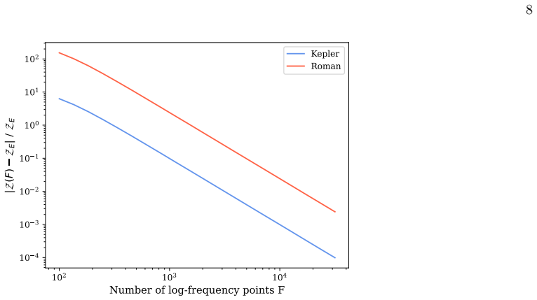
The central claim is that the inner-product precomputation scheme for Bayesian likelihoods, previously applied to pulsar timing residuals, carries over to coherent gravitational-wave astrometry essentially unchanged: for a constant-frequency source, the Gaussian log-likelihood of the deflection data is exactly a linear combination of a handful of inner products between the data and $\cos(\omega t)$/$\sin(\omega t)$ filters. Interpolating those inner products on a log-spaced frequency grid keeps the evidence accurate to within 1% for a barely detectable (Bayes factor $B=10$) source, provided enough grid points ($F=3140$ for Kepler, $F=15500$ for Roman). The paper demonstrates this with injection-based nested sampling runs and produces sensitivity forecasts: averaging over source sky positions, Kepler reaches $h_0 \geq 10^{-12.45}$ and Roman reaches $h_0 \geq 10^{-11.39}$ over $10^{-8}$ to $10^{-6}$ Hz, corresponding to detectability of a $10^9\,M_\odot$ chirp-mass binary at 3.6 Mpc (Kepler) or 0.31 Mpc (Roman).

Load-bearing premise

The pipeline assumes each candidate gravitational wave keeps a nearly constant frequency over the whole observing window, so that the signal is a pure sinusoid; if a real source's frequency evolves appreciably within that time, the precomputed inner products no longer represent the signal and the compressed likelihood is invalid in that part of the band.

Editorial extensions

If this is right

Coherent Bayesian searches of astrometric datasets with $10^5$–$10^8$ stars become computationally tractable, removing the hard-drive bottleneck that previously made MCMC or nested sampling infeasible.
Archival Kepler data and near-future Roman observations can be used to search the $10^{-8}$ to $10^{-6}$ Hz band, partially filling the gap between pulsar timing arrays and space-based interferometers.
The strong dependence of sensitivity on source–telescope separation means searches should marginalize over sky position; position-targeted strategies give only modest gains ($\Delta\log_{10} h_0 \approx -0.2$).
Frequency-targeted searches, using electromagnetic priors, are expected to improve sensitivity substantially, although the paper does not quantify that gain.
The compressed dataset retains per-baseline information (no averaging of stars), so the compression step does not mask spatially correlated systematics.

Reading between the lines

Editorial extensions of the paper, not claims the author makes directly.

One could extend the same precomputation to chirping signals by using a bank of frequency-evolution templates, interpolating over chirp mass as well as frequency, which would remove the main restriction at the high-frequency end.
The compression factor depends on the number of exposures per star, so future surveys with longer baselines or higher cadence will benefit even more, while very short surveys may not.
The same likelihood rewrite may apply to other high-baseline, low-SNR astrometric searches, such as exoplanet astrometry or searches for compact dark-matter lenses, wherever the signal is a coherent sinusoid in time.
If real microhertz sources chirp on month timescales, the quoted strain thresholds are optimistic; a direct search over $10^{-6}$–$10^{-4}$ Hz will need the chirping extension before claiming astrophysical constraints.

Share X Bluesky LinkedIn Reddit HN

Signed reviews

No signed human review yet.

Editorial analysis

A structured set of objections, weighed in public.

Desk editor's note, referee report, and a circularity audit.

Desk Editor's Note

read the letter

Two things to know up front. The compression method is real: transferring the PTA inner-product precomputation from Becsy et al. to astrometric deflections is a clean, non-obvious move, and the likelihood rewrite is algebraically sound. Second, the headline numbers should be read as order-of-magnitude forecasts, not hard sensitivities. The 1%-accuracy claim is supported at a single frequency, and the forecast pipeline makes optimistic noise/systematics choices that the authors disclose but do not fix.

What's genuinely new is applying this compression to relative astrometry, which opens a practical route into the microhertz band with Kepler and Roman data. The paper does a good job of laying out the survey models, the noise scaling, and the nested sampling setup. The finding that small fields of view make sky localization poor, and that targeted galaxy-position searches help only marginally, is a useful and non-obvious result. The authors are also refreshingly honest about the high-frequency end: avoiding frequency evolution forces unrealistically low chirp masses and sub-Mpc distances, and they say so.

The main soft spot is the accuracy claim. Section III A and Figure 2 measure interpolation error only at f=1e-7 Hz, and the F values that satisfy the 1% criterion there are then used across the entire 10^-8 to 10^-6 Hz prior. The stress-test concern is on target: the number of grid points per independent frequency bin drops by an order of magnitude as f increases, and the paper's own observation that per-sample evidence errors are always negative indicates the coarse grid systematically under-resolves narrow likelihood peaks. This is fixable, but it needs a multi-frequency error scan before the headline claim is credible.

Two lesser concerns. First, the forecasts assume white noise, full systematics removal, and no mean subtraction for Kepler; those are optimistic, though clearly labeled. Second, the empirical Bayes evidence correction in Section II E uses the posterior width to rescale the evidence; that is an ad hoc step that could bias the B=10 thresholds, though the injection calibration makes it acceptable for a first forecast. No code or data are provided, so nothing can be independently checked.

Who should read this: anyone working on astrometric GW detection or microhertz data analysis. The method is a stepping stone, not the final word. I would send it to peer review with a request for multi-frequency validation and a more careful treatment of the evidence correction. It deserves referee time, but it needs revision before the accuracy and sensitivity claims are taken at face value.

Referee Report

3 major / 4 minor

Summary. The paper extends the pulsar-timing-array inner-product precomputation scheme of Bécsy et al. to coherent gravitational-wave searches in relative astrometry. By rewriting the Gaussian likelihood as a linear combination of precomputed inner products between the astrometric data and sine/cosine filter functions, and by interpolating these inner products on a log-spaced frequency grid, the authors compress the dataset from O(NT) to O(NF). They validate the approximation by comparing the interpolated Bayesian evidence with an exact nested-sampling evidence calculation for an injected f_I = 10^-7 Hz source, reporting <1% evidence error at F = 3140 for Kepler and F = 15500 for Roman. They then use the compressed likelihood with JAXNS to forecast B = 10 strain thresholds across 10^-8 to 10^-6 Hz, obtaining h0 about 10^-12.45 for Kepler and about 10^-11.39 for Roman. The paper also reports poor sky localization and a marginal sensitivity gain from position-targeted searches.

Significance. If the accuracy claim is robust across the full frequency band, the compression step is a practical enabler for coherent microhertz astrometric searches on terabyte-scale datasets, and the Kepler/Roman forecasts provide concrete, falsifiable sensitivity targets. The method is an independent extension of existing PTA techniques, the nested-sampling setup is documented in sufficient detail for reproducibility, and the paper is transparent about the constant-frequency limitation. The main caveats are that the 1% accuracy is demonstrated at only one frequency, the quoted thresholds are for face-on binaries only, and the empirical-Bayes evidence correction is not calibrated; these issues affect the headline quantitative claims.

major comments (3)

[III.A and Figure 2] The headline claim that the compression is accurate 'to within 1% over two orders of magnitude in gravitational wave frequency' is supported by a single injected frequency, f_I = 10^-7 Hz, in Section III.A. For a log-spaced grid, the number of grid points per independent 1/T_obs frequency bin is proportional to (f_I T_obs)^-1. For Kepler (T_obs about 1.3e8 s), the F = 3140 grid has roughly 50 points per bin at f = 10^-7 Hz but only about 5 points per bin at f = 10^-6 Hz; for Roman (F = 15500) the corresponding drop is from about 800 to 90. The systematic negative per-sample evidence error noted by the authors indicates that under-resolved likelihood peaks are underestimated, so the same F cannot automatically be assumed accurate at the high-frequency end. Repeating the evidence-accuracy test at f_I = 10^-8 Hz and f_I = 10^-6 Hz, or deriving a frequency-dependent F requirement, is necessary to support the abstract's two-order-of-magnitude claim.
[III.B, Figure 3, and Abstract] The quoted B = 10 thresholds (h0 about 10^-12.45 for Kepler and about 10^-11.39 for Roman, used in the abstract and conclusion) are averages over sky position only; the full injection grid is run solely for face-on binaries (cos i = 1). The paper's own check at f_I = 10^-7 Hz for Kepler shows that the threshold worsens by Delta log10 h0 about 0.2 at cos i = 0.5 and by a similar amount from 45 degrees to edge-on. For a population with random inclinations, the average threshold strain would therefore be roughly 0.2-0.4 dex higher. The headline numbers should either be labeled as face-on, optimally oriented sensitivities, or the forecasts should marginalize over inclination.
[II.E and III.B] In Section II.E, the Bayesian evidence is corrected by multiplying Z_GW by 10^(W-N), where N is the 1-99% width of the h0 posterior obtained from the same data. This is an empirical-Bayes plug-in procedure rather than a Bayes factor under a fixed prior, and the null distribution of the resulting statistic is not characterized. Because the sensitivity thresholds in Section III.B are defined by B = 10, a calibration check with noise-only injections (or an analytic statement of the implied false-alarm rate) is needed to show that the correction does not distort the detection statistic. At minimum, the text should state explicitly that B is a corrected empirical-Bayes quantity rather than a proper Bayes factor.

minor comments (4)

[III.A and Figure 2] Each curve in Figure 2 comes from a single nested-sampling run, so the F values quoted for 1% accuracy have no associated uncertainty; a few independent realizations would make the threshold more robust.
[III.A] The statement that the evidence error does not depend on the number of observations per star or on the signal-to-noise ratio is asserted without a supporting test; since this scaling is later used to justify F = 1000 in Section III.B, it should be demonstrated explicitly.
[III.B] The substitution of N_sub = 1000 stars with scaled-down noise for the full catalog is described in one sentence; a single full-star run at one frequency would confirm that the scaling preserves both the sensitivity and the interpolation accuracy.
[III.B and Figure 3] The dashed high-frequency extrapolation to 10^-3.5 Hz is not used for the quoted thresholds; given the text's own caveat that this regime requires frequency-evolution-aware methods, consider removing it or labeling it more prominently as an illustration.

Circularity Check

0 steps flagged · score 1.0 of 10

No significant circularity: the compression method, accuracy test, and injection-based forecasts are self-contained and do not reduce to their inputs.

full rationale

The derivation chain is self-contained. The inner-product compression is an exact algebraic rewrite of the Gaussian likelihood (Section II C), inherited from the external PTA work [20,21]; the astrometric extension is then tested by comparing the approximate evidence Z(F) against the exact evidence Z_E on injected mock data (Section III A, Figure 2), which is a direct numerical accuracy test rather than a fitted prediction. The sensitivity thresholds in Section III B come from injected signals and nested-sampling Bayes factors, so they are not renamed inputs. The only self-citations ([17-19]) supply survey parameters and mean-subtraction factors; they are assumptions, not the conclusion, and they do not force the compression or the threshold results. Section II E's post-hoc evidence rescaling uses the h0 posterior width from the same data and is acknowledged as empirical Bayes; while this makes the detection statistic partially data-defined and could affect the absolute B=10 thresholds, it is not an equation-level reduction of a prediction to an input. The abstract's '1% over two orders of magnitude' claim is directly tested only at f_I=10^-7 Hz (Section III A, Figure 2), so the band-wide accuracy is an extrapolation; this is a support gap and correctness risk, not circularity. No circular step is exhibited.

Assumptions & free parameters 3 free parameters · 6 assumptions · 0 invented entities

The central compression method rests on constant-frequency sinusoids and the observer-term-only response. The forecasts add assumptions about white noise, systematics removal, mean-signal subtraction, and Newtonian circular binaries. The post-hoc evidence correction is the only data-fitted quantity in the pipeline. No invented physical entities are needed.

free parameters (3)

Frequency grid point count F = 3140 (Kepler), 15500 (Roman) for 1% exact evidence; 1000 in search runs
Interpolation grid density controls approximation error; F=1000 is used on noise-scaled 1000-star subsets and justified by sqrt(N) error scaling (Section III A).
Post-hoc h0 evidence correction factor = 10^(W-N) with W=7 and N the 1%-99% h0 posterior extent, varies per run
Section II E: the evidence is multiplied by this factor to emulate an empirically chosen h0 prior; N is measured from the same posterior, so the correction is data-fitted.
Noise scaling for star subsets = sqrt(Nsub/Nall) about 12.6 for Kepler, 316 for Roman
Section III B: 1000-star subsets with per-star noise scaled down are used to represent the full surveys; assumes identical independent noise.

assumptions (6)

domain assumption The GW frequency f_I is constant over the observation window, so the signal is a linear combination of cos(omega t) and sin(omega t).
Required for the likelihood rewrite in Section II C; the forecasts enforce it by capping chirp mass at each frequency (Section III B), and the conclusion states this is the primary limitation.
domain assumption Only the observer term in Eq. (1) matters; the star term is treated as additional stochastic noise.
Section II A assumes stars are at different distances so source-term deflections are uncorrelated; if not, the likelihood model omits a coherent component.
domain assumption Astrometric noise is white, independent across stars, and all systematics are fully removed, with Kepler unaffected by mean-signal subtraction.
Section II B states these are optimistic assumptions used for the mock data and forecasts.
domain assumption Flat-sky approximation fixes tangent vectors to the field-of-view center for all stars.
Section II B; for Kepler's 105 deg^2 field this can introduce geometric errors at the field edges.
domain assumption Roman is modeled in the full mean-subtraction regime, equivalent to a factor of 100 increase in noise.
Section III B and Refs. [17-19]; this drives Roman's lower sensitivity.
domain assumption The gravitational wave source is a circular binary in the Newtonian 0PN approximation, with h-tensor given by Eq. (2).
Used throughout the mock data generation and likelihood; higher-order corrections or eccentricity are ignored.

how reviews work

0 comments

Cite this review

Pith. "Pith review of A Fast Bayesian Method for Coherent Gravitational Wave Searches with Relative Astrometry." pith.science (2026). https://pith.science/paper/DRSMRUTH

@misc{pith2026250619206,
  author       = {Pith},
  title        = {Pith review of: A Fast Bayesian Method for Coherent Gravitational Wave Searches with Relative Astrometry},
  year         = {2026},
  howpublished = {\url{https://pith.science/paper/DRSMRUTH}},
  note         = {Machine review of arXiv:2506.19206}
}

abstract

Using relative stellar astrometry for the detection of coherent gravitational wave sources is a promising method for the microhertz range, where no dedicated detectors currently exist. Compared to other gravitational wave detection techniques, astrometry operates in an extreme high-baseline-number and low-SNR-per-baseline limit, which leads to computational difficulties when using conventional Bayesian search techniques. We extend a technique for efficiently searching pulsar timing array datasets through the precomputation of inner products in the Bayesian likelihood, showing that it is applicable to astrometric datasets. Using this technique, we are able to reduce the total dataset size by up to a factor of $\mathcal{O}(100)$, while remaining accurate to within 1% over two orders of magnitude in gravitational wave frequency. Applying this technique to simulated astrometric datasets for the Kepler Space Telescope and Nancy Grace Roman Space Telescope missions, we obtain forecasts for the sensitivity of these missions to coherent gravitational waves. Due to the low angular sky coverage of astrometric baselines, we find that coherent gravitational wave sources are poorly localized on the sky. Despite this, from $10^{-8}$ Hz to $10^{-6}$ Hz, we find that Roman is sensitive to coherent gravitational waves with an instantaneous strain above $h_0 \simeq 10^{-11.4}$, and Kepler is sensitive to strains above $h_0 \simeq $ $10^{-12.4}$. At this strain, we can detect a source with a frequency of $10^{-7}$ Hz and a chirp mass of $10^9$ $M_\odot$ at a luminosity distance of 3.6 Mpc for Kepler, and 0.3 Mpc for Roman.

Figures

Figures reproduced from arXiv: 2506.19206 by the authors.

**Figure 2.** FIG. 2: Relative error in the Bayesian evidence [PITH_FULL_IMAGE:figures/full_fig_p008_2.png] view at source ↗

**Figure 3.** FIG. 3: Position-averaged instantaneous strain sensitivity for [PITH_FULL_IMAGE:figures/full_fig_p010_3.png] view at source ↗

Figures from the paper (2 more)

**Figure 4.** Figure 4: FIG. 4: Corner plot of an individual nested sampling run for [PITH_FULL_IMAGE:figures/full_fig_p011_4.png]

**Figure 5.** Figure 5: FIG. 5: Polar-projection plot of maximum likelihood versus source position, for a [PITH_FULL_IMAGE:figures/full_fig_p013_5.png]

Review history (2 revisions) →

Discussion (0). Continue with ORCID to comment.

Reference graph

Works this paper leans on

44 extracted references · 26 canonical work pages

[1]

B. P. Abbott, R. Abbott, T. D. Abbott,et al., Phys. Rev. D93, 122003 (2016), arXiv:1602.03839 [gr- qc]

arXiv 2016
[2]

Agazie, A

G. Agazie, A. Anumarlapudi, A. M. Archibald,et al., The Astrophysical Journal Letters951, L8 (2023)

work page 2023
[3]

Anto- niadis, P

EPTA Collaboration and InPTA Collaboration:, J. Anto- niadis, P. Arumugam,et al., Astronomy & Astrophysics 678, A50 (2023)

work page 2023
[4]

However, explicitly confirming this result for coherent GW searches using astrometric deflections is beyond the scope of this work. IV. CONCLUSION In this work, we explore the prospects of detect- ing coherent gravitational wave sources from theKe- plerandRomanphotometric surveys, using relative stellar astrometry. Unlike any other GW detection method, fo...

work page 2024
[5]

D. J. Reardon, A. Zic, R. M. Shannon,et al., The Astro- physical Journal Letters951, L6 (2023)

work page 2023
[6]

H. Xu, S. Chen, Y. Guo,et al., Research in Astronomy and Astrophysics23, 075024 (2023)

work page 2023
[7]

Agazie, P

G. Agazie, P. T. Baker, B. B´ ecsy,et al., The NANOGrav 15 yr Data Set: Looking for Signs of Dis- creteness in the Gravitational-wave Background (2024), arXiv:2404.07020 [astro-ph]

arXiv 2024
[8]

Afzal, G

A. Afzal, G. Agazie, A. Anumarlapudi,et al., ApJ951, L11 (2023), arXiv:2306.16219 [astro-ph.HE]

arXiv 2023

Show all 44 references

[9]

Amaro-Seoane, H

P. Amaro-Seoane, H. Audley, S. Babak,et al., Laser Interferometer Space Antenna (2017), arXiv:1702.00786 [astro-ph]

2017 arXiv
[10]

Agazie, A

G. Agazie, A. Anumarlapudi, A. M. Archibald,et al., The Astrophysical Journal Letters951, L50 (2023), arXiv:2306.16222 [astro-ph, physics:gr-qc]. 14

2023 arXiv
[11]

Chang and Y

C.-F. Chang and Y. Cui, Physics of the Dark Universe 29, 100604 (2020)

2020
[12]

Colpi, K

M. Colpi, K. Danzmann, M. Hewitson,et al., LISA Defi- nition Study Report (2024), arXiv:2402.07571 [astro-ph, physics:gr-qc]

2024 arXiv
[13]

T. Pyne, C. R. Gwinn, M. Birkinshaw,et al., The Astro- physical Journal465, 566 (1996)

1996
[14]

Dom` enech and M

G. Dom` enech and M. Sasaki, Classical and Quantum Gravity41, 143001 (2024)

2024
[15]

S. A. Klioner, Classical and Quantum Gravity35, 045005 (2018)

2018
[16]

L. G. Book and E. E. Flanagan, Physical Review D83, 024024 (2011)

2011
[17]

Y. Wang, K. Pardo, T.-C. Chang, and O. Dor´ e, Phys. Rev. D103, 084007 (2021), arXiv:2010.02218 [gr- qc]

2021 arXiv
[18]

C. J. Moore, D. P. Mihaylov, A. Lasenby, and G. Gilmore, Physical Review Letters119, 261102 (2017)

2017
[19]

Pardo, T.-C

K. Pardo, T.-C. Chang, O. Dor´ e, and Y. Wang, Gravi- tational Wave Detection with Relative Astrometry using Roman’s Galactic Bulge Time Domain Survey (2023), version Number: 1

2023
[20]

Y. Wang, K. Pardo, T.-C. Chang, and O. Dor´ e, Phys. Rev. D106, 084006 (2022), arXiv:2205.07962 [gr- qc]

2022 arXiv
[21]

B´ ecsy, arXiv e-prints , arXiv:2406.16331 (2024), arXiv:2406.16331 [gr-qc]

B. B´ ecsy, arXiv e-prints , arXiv:2406.16331 (2024), arXiv:2406.16331 [gr-qc]

2024 arXiv
[22]

B´ ecsy, N

B. B´ ecsy, N. J. Cornish, and M. C. Digman, Phys. Rev. D 105, 122003 (2022), arXiv:2204.07160 [gr-qc]

2022 arXiv
[23]

B. S. Gaudi and D. P. Bennett, Roman White Papers - 2023 (2023)

2023
[24]

Aghanim, Y

Planck Collaboration, N. Aghanim, Y. Akrami,et al., Astronomy & Astrophysics641, A6 (2020)

2020
[25]

W. J. Borucki, D. Koch, G. Basri,et al., Science327, 977 (2010)

2010
[26]

B. S. Gaudi, R. Akeson, J. Anderson,et al., ”Auxiliary” Science with the WFIRST Microlensing Survey (2019), version Number: 1

2019
[27]

D. G. Monet, J. M. Jenkins, E. W. Dunham,et al., Pre- liminary Astrometric Results from Kepler (2010), version Number: 1

2010
[28]

J. E. Van Cleve, J. L. Christiansen, J. M. Jenkins, et al., Kepler Data Characteristics Handbook, Kepler Sci- ence Document KSCI-19040-005, id. 2. Edited by Doug Caldwell, Jon M. Jenkins, Michael R. Haas and Natalie Batalha (2016)

2016
[29]

Vallenari, A

Gaia Collaboration, A. Vallenari, A. G. A. Brown,et al., A&A674, A1 (2023), arXiv:2208.00211 [astro-ph.GA]

2023 arXiv
[30]

T. M. Brown, D. W. Latham, M. E. Everett, and G. A. Esquerdo, AJ142, 112 (2011), arXiv:1102.0342 [astro- ph.SR]

2011 arXiv
[31]

WFIRST Astrometry Working Group, R. E. Sander- son, A. Bellini,et al., Journal of Astronomical Tele- scopes, Instruments, and Systems5, 044005 (2019), arXiv:1712.05420 [astro-ph.IM]

2019
[32]

K. A. Janes, ApJ835, 75 (2017), arXiv:1612.00070 [astro-ph.SR]

2017 arXiv
[33]

Bradbury, R

J. Bradbury, R. Frostig, P. Hawkins,et al., JAX: com- posable transformations of Python+NumPy programs (2024)

2024
[34]

Skilling, Bayesian Analysis1, 833 (2006)

J. Skilling, Bayesian Analysis1, 833 (2006)

2006
[35]

J. G. Albert, arXiv e-prints , arXiv:2312.11330 (2023), arXiv:2312.11330 [astro-ph.IM]

2023 arXiv
[36]

J. G. Albert, arXiv e-prints , arXiv:2012.15286 (2020), arXiv:2012.15286 [astro-ph.IM]

2020 arXiv
[37]

Llorente, L

F. Llorente, L. Martino, E. Curbelo,et al., arXiv e-prints , arXiv:2206.05210 (2022), arXiv:2206.05210 [stat.ME]

2022 arXiv
[38]

R. E. Kass and A. E. Raftery, Journal of the American Statistical Association90, 773 (1995)

1995
[39]

Arzoumanian, P

Z. Arzoumanian, P. T. Baker, A. Brazier,et al., ApJ900, 102 (2020), arXiv:2005.07123 [astro-ph.GA]

2020 arXiv
[40]

The authors also acknowledge the Center for Ad- vanced Research Computing (CARC) at the University of Southern California for providing computing resources that have contributed to the research results reported within this publication. Part of this work was done at Jet Propuls...
[41]

Petrone, S

S. Petrone, S. Rizzelli, J. Rousseau, and C. Scricciolo, METRON72, 201 (2014)

2014
[42]

Antil, S

H. Antil, S. E. Field, F. Herrmann,et al., arXiv e-prints , arXiv:1210.0577 (2012), arXiv:1210.0577 [cs.NA]

2012 arXiv
[43]

Leslie, L

N. Leslie, L. Dai, and G. Pratten, Physical Review D 104, 123030 (2021)

2021
[44]

N. J. Cornish, Physical Review D104, 104054 (2021)

2021

Pith tools

Reviewed August 15, 2026 · model on record in the stance chip above.

[1] [1]

B. P. Abbott, R. Abbott, T. D. Abbott,et al., Phys. Rev. D93, 122003 (2016), arXiv:1602.03839 [gr- qc]

arXiv 2016

[2] [2]

Agazie, A

G. Agazie, A. Anumarlapudi, A. M. Archibald,et al., The Astrophysical Journal Letters951, L8 (2023)

work page 2023

[3] [3]

Anto- niadis, P

EPTA Collaboration and InPTA Collaboration:, J. Anto- niadis, P. Arumugam,et al., Astronomy & Astrophysics 678, A50 (2023)

work page 2023

[4] [4]

However, explicitly confirming this result for coherent GW searches using astrometric deflections is beyond the scope of this work. IV. CONCLUSION In this work, we explore the prospects of detect- ing coherent gravitational wave sources from theKe- plerandRomanphotometric surveys, using relative stellar astrometry. Unlike any other GW detection method, fo...

work page 2024

[5] [5]

D. J. Reardon, A. Zic, R. M. Shannon,et al., The Astro- physical Journal Letters951, L6 (2023)

work page 2023

[6] [6]

H. Xu, S. Chen, Y. Guo,et al., Research in Astronomy and Astrophysics23, 075024 (2023)

work page 2023

[7] [7]

Agazie, P

G. Agazie, P. T. Baker, B. B´ ecsy,et al., The NANOGrav 15 yr Data Set: Looking for Signs of Dis- creteness in the Gravitational-wave Background (2024), arXiv:2404.07020 [astro-ph]

arXiv 2024

[8] [8]

Afzal, G

A. Afzal, G. Agazie, A. Anumarlapudi,et al., ApJ951, L11 (2023), arXiv:2306.16219 [astro-ph.HE]

arXiv 2023