REVIEW 4 major objections 4 minor 26 references
Pseudorandom streams consumed by a diffusion model act as model-dependent structured inputs, shifting training loss and generation quality even after marginal statistics are controlled.
Reviewed by Pith at T0; open to challenge. T0 means a machine referee read the full paper against a public rubric. the ladder, T0–T4 →
T0 review · deepseek-v4-flash
2026-08-04 04:25 UTC pith:DSLOAFPD
load-bearing objection A careful, honest empirical study showing that PRNG orbit choice is a model-dependent variable for diffusion training, but the quantitative power law rests on a small screened sample and the comparison with conventional statistical indicators is deferred. the 4 major comments →
Pseudorandom Streams within Diffusion Models Act as Learnable Inputs That Affect Generation Quality
The pith
A machine-rendered reading of the paper's core claim, the machinery that carries it, and where it could break.
Core claim
On its own terms, the paper's central claim is that a pseudorandom source is not only a distributional choice but also a model-dependent structured input. The realized training objective depends on the concrete values consumed at each step, and gradient descent can exploit accessible orbit structure exactly as it exploits regularities in data. As evidence, the paper shows that after rank uniformization, Box–Muller Gaussianization, and mean–variance calibration remove marginal differences, and after pre-screening removes period-two band alternation and finite-precision absorbing states, the surviving Logistic, Markov-type, and ShiftedSine orbits still split diffusion training into clearly dif
What carries the argument
The load-bearing object is the concrete pseudorandom orbit—a finite-precision numerical trajectory jointly determined by a recurrence, its parameters, an initial state, and rounding—treated as part of the optimization argument. The argument flows through the realized loss L_t(theta_t; D, R_t) and its gradient; because every update consumes concrete values from R_t, any structure a network can learn to exploit reduces the realized objective independently of the data. The paper's two operational probes are the MLP next-value predictor (one hidden layer, width 8, 273 parameters, input of the 32 previous uniformized values; the IID floor for prediction loss is 1/12) and the diffusion probe (same
Load-bearing premise
The conclusion rests on the assumption that, after the pipeline of rank uniformization, Box–Muller Gaussianization, mean–variance calibration, and screening out band alternation and absorbing states, the remaining cross-source differences in diffusion loss and generation quality come from temporal structure that the tested systems can exploit—not from some unmeasured conventional statistical deviation (such as higher-order marginals, lag-k dependence, or spectral content) tha
What would settle it
Compute conventional statistics on the Gaussianized, uniformized orbits—for example lag-1 and lag-2 autocorrelation, mutual information between consecutive values, spectral flatness, or a standard test battery applied to the uniformized sequence—and measure their Spearman rank correlation with the human generation grades against the probe's roughly 0.93. If any standard statistic matches or exceeds that correlation and also predicts real-data diffusion loss under the same IID normalization, the claim that the effect is due to model-relative 'learnable' orbit structure rather than any deviation
If this is right
- PRNG evaluation for machine learning should include model-relative exploitability, not just conventional statistical test suites.
- Lower training loss can accompany worse generation quality, because the optimizer may be fitting the random stream rather than the data.
- The diffusion probe is a cheap ranking instrument for random sources before committing to expensive full real-data training runs.
- Larger models and more random calls may make weaker orbit structures exploitable, so industrial PRNGs should be re-checked at scale.
- Mixing source types between training and sampling defines a different configuration, so source consistency matters for reproducible generation.
Where Pith is reading between the lines
- If the mechanism generalizes, the PRNG family and its seed become effectively hyperparameters of the generative model, and reproducible ML reports would need to state them explicitly alongside architecture and data.
- A direct causal test would shuffle each surviving orbit within short blocks (e.g., length 32) while preserving its marginals; if the spread in diffusion loss and generation grades collapses toward the IID baseline, temporal order is the carrier of the effect.
- The system-dependent exponent rho could be measured across model capacities, batch sizes, or noise schedules; if it varies smoothly, it might serve as a practical 'learnability calibration' for how strongly a diffusion system responds to the random source.
Editorial analysis
A structured set of objections, weighed in public.
Referee Report
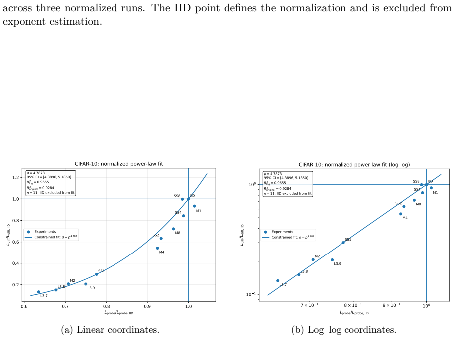
Summary. The paper studies whether the concrete pseudorandom orbit consumed by a diffusion model can act as a model-dependent 'learnable input' that affects training loss and generation quality. After applying empirical-rank uniformization, Box–Muller Gaussianization, and mean–variance calibration to deterministic Logistic, Markov-type, Sine, and ShiftedSine orbits, and after screening out band-alternating and finite-precision-absorbing failures, the authors train U-Net diffusion models on MNIST and CIFAR-10 with each source as a continuous stream. They measure orbit predictability with a small MLP next-value predictor and 'exploitability' with a diffusion probe that replaces real images with online random tensors. Both indicators rank-correlate strongly with an ordered human grade of generated-image degradation, and the IID-normalized probe loss and real-data diffusion loss are reported to follow an empirical power law d = p^ρ, with ρ ≈ 3.06 on MNIST and ρ ≈ 4.79 on CIFAR-10. The paper concludes that pseudorandom sources are not just distributional choices but structured inputs whose effect is learning-system-dependent.
Significance. If the central observation is robust, the paper makes a useful and timely point: practical diffusion pipelines can be sensitive to the concrete PRNG implementation even after standard marginal statistics are controlled. The probe methodology is modular and could become a cheap screening instrument for PRNG quality in model-specific settings. The paper is also unusually careful in disclosing its limitations, and it provides code and data. The main scientific value is the empirical demonstration of strong, reproducible differences across a small set of screened orbits, together with a candidate quantitative relation (the power law) that—if confirmed on more runs and source families—would be a useful calibration. However, the current evidence is not yet sufficient to elevate the power law beyond a descriptive fit, and the absence of any conventional statistical baseline leaves the 'learnable input' attribution underdetermined.
major comments (4)
- [§5 (text before §5.1)] The manuscript explicitly defers the comparison with traditional statistical and dynamical indicators: 'A systematic comparison with traditional statistical and dynamical indicators is left for future work.' This is load-bearing for Contribution 2, which claims to go 'beyond conventional generator-level statistical quality.' Since the pipeline controls only the univariate marginal and mean/variance (§3.1), the remaining cross-source differences could be captured by conventional quantities such as lag-k autocorrelation, AR residual variance, spectral content, or TestU01 statistics. I ask that you compute a set of standard indicators on the same uniformized/Gaussianized screened orbits and report their Spearman correlations with the human grade and with the probe loss. If a conventional indicator matches the MLP/probe at Spearman ≈ 0.9, the 'learnable input' interpretation is underdetermin
- [§5.3, Eqs. (29)–(38), Fig. 4] The CIFAR-10 exponent ρ = 4.79 is estimated from matched run 1 only; Fig. 4 shows no run-to-run error bars, and §5.4 states that a second CIFAR-10 probe run was used only for ranking stability. The reported 95% CI is the residual-based interval of the zero-intercept regression and does not capture run-to-run variation in either the real-data diffusion loss or the probe loss. With n = 11 and a single matched run, the abstract's wording 'approximately follow an empirical power law, with different exponents on the two datasets' overstates the evidence. Please add independent matched CIFAR-10 runs or explicitly relabel this as a single-run descriptive relation with appropriate uncertainty.
- [§4 and §5.3] The power law is fitted to the same screened point set on which the qualitative phenomenon was established. The screening removes three grade-0 orbits (L3.6, Sine-1, L4.0), and the zero-intercept IID normalization anchors the curve through (1,1) by construction. The most extreme points L3.7 and L3.8 dominate the exponent estimate, making the fit sensitive to the screening decision. Please report leave-one-out exponent stability, a free-intercept fit, and the resulting exponent if one or more screened sources are re-included, to demonstrate that the power law is not an artifact of the exclusion rule.
- [§5.1.2 and §5.3] The probe loss and the real-data diffusion loss are not independent measurements: both use the same U-Net, the same noise-prediction objective, the same optimizer, and the same tested source, with the probe differing only in that clean images are replaced by random tensors. The empirical relation d = p^ρ may therefore reflect a shared dependence of both quantities on source-specific effective stochasticity, rather than a law connecting two genuinely distinct observables. The formalization in Eqs. (42)–(44) provides a useful language but does not resolve this. Please state explicitly what scientific content the power law adds beyond the shared monotonic association, and, if possible, test whether the relation is stable when the probe changes architecture or random-role configuration.
minor comments (4)
- [Table 3] Please state the sample size (n = 12) and the tie-handling procedure directly in the table caption. The exact permutation p-values are appropriate, but readers should not have to infer the sample size from the text.
- [Figs. 3 and 4] The axis tick labels in the log–log panels appear garbled in the manuscript rendering (e.g., '1006 × 10 1' and '1007 × 10 1'). Please correct these to the intended scientific notation, e.g., 10^{-1} and 10^{0}.
- [§5.4, Eq. (42)] The ideal-IID-referenced exploitability A_M(s) is defined with an oracle that 'cannot be implemented exactly by a finite deterministic digital algorithm,' yet the subsequent relative measure is used experimentally. Consider adding one sentence clarifying that A_M is a theoretical limiting object and that all empirical comparisons use the operational NumPy baseline, to avoid confusion about whether Eq. (42) is measured.
- [§5.4, Eqs. (40)–(41)] The MLP and probe loss Spearman correlations are very high (0.92), while the claim that 'local rankings differ' rests on small numerical differences. A small rank-difference table or a description of which sources change rank by more than one position would help the reader evaluate the distinctness of the two characterizations.
Circularity Check
No significant circularity: the power law is an explicitly in-sample empirical fit, and the neural indicators are independent measurements, not fitted to the outcomes they are compared with.
full rationale
The paper's central quantitative claims are either direct empirical measurements or descriptive fits to those measurements. The power-law relation (Eqs. 27-32) is a zero-intercept least-squares fit on the same screened sources, but the paper is transparent about this: it excludes the IID anchor from the exponent estimate, reports the fit quality, and frames the result as an empirical calibration ('working hypothesis rho = rho(M,D)'), not as an out-of-sample prediction or a first-principles derivation. The rank correlations use an MLP test loss evaluated on a held-out interval and a diffusion probe trained on semantically empty random tensors; neither indicator is fitted to the human grades or to the real-data diffusion loss, so there is no fitted-input-called-prediction step. The Section 4 screening removes orbits on a priori dynamical and finite-precision grounds (band alternation, absorbing states), not on the basis of the outcome variables. The paper itself flags the lack of comparison with conventional statistical and dynamical indicators ('A systematic comparison with traditional statistical and dynamical indicators is left for future work,' Section 5); that is a limitation on the distinctiveness of the 'learnable input' interpretation, but it is not a circular reduction. No equation is shown to be equivalent to its own input by construction, and no load-bearing result is imported from author self-citation. Thus no significant circularity is present.
Axiom & Free-Parameter Ledger
free parameters (4)
- power-law exponent rho (per dataset) =
3.0628 (MNIST), 4.7873 (CIFAR-10)
- screened source set (exclusion cut) =
12 of 14 orbits retained
- generator-family parameters (a, k, c) =
a in {3.6,3.7,3.8,3.9,4.0}; k in {2,4,8}; c=0.36787944117144233
- MLP and probe hyperparameters =
MLP width 8 (273 params), history 32, up to 5000 steps; MNIST 30 epochs; CIFAR-10 30000 steps
axioms (6)
- domain assumption After empirical-rank uniformization + Box-Muller + mean-variance calibration, cross-source differences are attributable to temporal orbit structure, not residual marginal statistics
- domain assumption NumPy default PRNG is an operational IID reference with no exploitable structure under these models
- domain assumption Excluded orbits (L3.6, Sine-1, L4.0) are genuine failures outside the continuous learnability spectrum
- domain assumption Ordered human grades are a valid macroscopic quality measure for rank correlation
- domain assumption MLP next-value MSE and diffusion-probe tail loss operationalize 'learnability'
- standard math Taylor-expansion capture-range analysis for finite-precision absorption (Eqs. 8-12)
read the original abstract
Diffusion models rely on stochastic inputs, yet on finite-precision hardware, the "randomness" they consume is realized as deterministic numerical orbits generated by pseudorandom rules. Accessible orbit structure can become a learnable input and affect both training and generation because the realized loss and its gradient depend on the concrete pseudorandom values consumed at each optimization step. A small multilayer perceptron predicts the next value of an orbit from its recent history, measuring general sequence predictability. A diffusion probe replaces real images with online random tensors while preserving the diffusion architecture and training objective, measuring whether the target system can exploit orbit structure. After controlling marginal statistics and screening out clear dynamical and finite-precision failures, the remaining orbits still produce markedly different diffusion losses and generation quality on MNIST and CIFAR-10. Both measures show strong rank correlations with macroscopic generation degradation, although their local rankings differ. After normalization by the IID baseline, the probe loss and the real-data diffusion loss approximately follow an empirical power law, with different exponents on the two datasets. These results suggest that a pseudorandom source is not only a distributional choice, but also a model-dependent structured input.
Figures




Reference graph
Works this paper leans on
-
[1]
Denoising Diffusion Probabilistic Models,
J. Ho, A. Jain, and P. Abbeel, “Denoising Diffusion Probabilistic Models,”Advances in Neural Information Processing Systems, vol. 33, pp. 6840–6851, 2020
2020
-
[2]
A. J. Menezes, P. C. van Oorschot, and S. A. Vanstone,Handbook of Applied Cryptography. Boca Raton, FL, USA: CRC Press, 1996, Chapter 5
1996
-
[3]
TestU01: A C library for empirical testing of random number generators,
P. L’Ecuyer and R. Simard, “TestU01: A C library for empirical testing of random number generators,”ACM Transactions on Mathematical Software, vol. 33, no. 4, Article 22, 2007
2007
-
[4]
Rukhin, J
A. Rukhin, J. Soto, J. Nechvatal, et al.,A Statistical Test Suite for Random and Pseudoran- dom Number Generators for Cryptographic Applications. NIST Special Publication 800-22 Rev. 1a, 2010
2010
-
[5]
Learning from pseudo-randomness with an artificial neural network— Does God play pseudo-dice?
F. Fan and G. Wang, “Learning from pseudo-randomness with an artificial neural network— Does God play pseudo-dice?” arXiv:1801.01117, 2018
Pith/arXiv arXiv 2018
-
[6]
(How) can Transformers predict pseudo-random numbers?
T. Tao, D. Doshi, D. S. Kalra, T. He, and M. Barkeshli, “(How) can Transformers predict pseudo-random numbers?” arXiv:2502.10390, 2025
Pith/arXiv arXiv 2025
-
[7]
T. Tao and M. Barkeshli, “Learning pseudorandom numbers with Transformers: Permuted congruential generators, curricula, and interpretability,” arXiv:2510.26792, 2025
Pith/arXiv arXiv 2025
-
[8]
Non-Gaussian denoising diffusion models,
E. Nachmani, R. San Roman, and L. Wolf, “Non-Gaussian denoising diffusion models,” arXiv:2106.07582, 2021. 21
Pith/arXiv arXiv 2021
-
[9]
Score-based denoising diffusion with non-isotropic Gaussian noise models,
V. Voleti, C. Pal, and A. Oberman, “Score-based denoising diffusion with non-isotropic Gaussian noise models,” arXiv:2210.12254, 2022
Pith/arXiv arXiv 2022
-
[10]
Blue noise for diffusion models,
X. Huang, C. Salaün, C. Vasconcelos, C. Theobalt, C. Öztireli, and G. Singh, “Blue noise for diffusion models,”ACM SIGGRAPH Conference Papers, 2024
2024
-
[11]
Good seed makes a good crop: Discovering secret seeds in text-to-image diffusion models,
K. Xu, L. Zhang, and J. Shi, “Good seed makes a good crop: Discovering secret seeds in text-to-image diffusion models,”Proceedings of the IEEE/CVF Winter Conference on Applications of Computer Vision, pp. 3024–3034, 2025
2025
-
[12]
Ott,Chaos in Dynamical Systems, 2nd ed
E. Ott,Chaos in Dynamical Systems, 2nd ed. Cambridge, UK: Cambridge University Press, 2002
2002
-
[13]
N. J. Higham,Accuracy and Stability of Numerical Algorithms, 2nd ed. Philadelphia, PA, USA: SIAM, 2002
2002
-
[14]
On the dynamical degradation of digital piecewise linear chaotic maps,
S. Li, G. Chen, and X. Mou, “On the dynamical degradation of digital piecewise linear chaotic maps,”International Journal of Bifurcation and Chaos, vol. 15, no. 10, pp. 3119–3151, 2005
2005
-
[15]
Periodic orbits in chaotic systems simulated at low precision,
M. Klöwer, P. V. Coveney, E. A. Paxton, and T. N. Palmer, “Periodic orbits in chaotic systems simulated at low precision,”Scientific Reports, vol. 13, Article 11410, 2023
2023
-
[16]
Gradient-based learning applied to document recognition,
Y. LeCun, L. Bottou, Y. Bengio, and P. Haffner, “Gradient-based learning applied to document recognition,”Proceedings of the IEEE, vol. 86, no. 11, pp. 2278–2324, 1998
1998
-
[17]
Krizhevsky,Learning Multiple Layers of Features from Tiny Images
A. Krizhevsky,Learning Multiple Layers of Features from Tiny Images. Technical Report, University of Toronto, 2009
2009
-
[18]
Diffusers training overview and unconditional image generation training guide,
Hugging Face, “Diffusers training overview and unconditional image generation training guide,” online documentation, accessed July 26, 2026
2026
-
[19]
google/ddpm-cifar10-32: UNet2DModel configuration,
Hugging Face and Google, “google/ddpm-cifar10-32: UNet2DModel configuration,” online model configuration, accessed July 27, 2026
2026
-
[20]
A note on the generation of random normal deviates,
G. E. P. Box and M. E. Muller, “A note on the generation of random normal deviates,”The Annals of Mathematical Statistics, vol. 29, no. 2, pp. 610–611, 1958
1958
-
[21]
Lapedes and R
A. Lapedes and R. Farber,Nonlinear Signal Processing Using Neural Networks: Prediction and System Modelling. Los Alamos National Laboratory Report LA-UR-87-2662, 1987
1987
-
[22]
Deep learning scaling is predictable, empirically,
J. Hestness, S. Narang, N. Ardalani, et al., “Deep learning scaling is predictable, empirically,” arXiv:1712.00409, 2017
Pith/arXiv arXiv 2017
-
[23]
Auto-encoding variational Bayes,
D. P. Kingma and M. Welling, “Auto-encoding variational Bayes,” arXiv:1312.6114, 2013
Pith/arXiv arXiv 2013
-
[24]
Denoising diffusion implicit models,
J. Song, C. Meng, and S. Ermon, “Denoising diffusion implicit models,”International Conference on Learning Representations, 2021
2021
-
[25]
B. A. Antunes, “Statistical quality and reproducibility of pseudorandom number generators in machine learning technologies,” arXiv:2507.03007, 2025
Pith/arXiv arXiv 2025
-
[26]
B. A. Antunes, “The influence of the random numbers quality on the results in stochastic simulations and machine learning,” arXiv:2510.25269, 2025. 22
arXiv 2025
discussion (0)
Sign in with ORCID, Apple, or X to comment. Anyone can read and Pith papers without signing in.