Kernel Stochastic Configuration Networks for Nonlinear Regression

Dianhui Wang; Yongxuan Chen

REVIEW 3 major objections 5 minor 35 references

Kernel Stochastic Configuration Networks for Nonlinear Regression

T0 review · 3 major / 5 minor · reviewed 2026-08-11 · deepseek-v4-flash

Challenge this review Re-run · record.json Download PDF Read on arXiv ↗ Review JSON

Pith's one-line read KSCNs preserve the universal approximation property of SCNs while improving regression accuracy and stability across benchmark and industrial datasets.

desk verdict KSCN is a plausible new kernel construction with real but modest empirical gains, but the universal approximation proof in Theorem 1 does not hold as written. read the letter →

arxiv 2412.05846 v2 pith:DTT3HARV submitted 2024-12-08 cs.LG cs.AI

Yongxuan Chen , Dianhui Wang This is my paper · ORCID

classification cs.LGcs.AI MSC 68T0768T0568Q32

keywords kernelstochasticconfigurationnetworksrandomizedneuraluniversalapproximationreproducingHilbertspacenonlinearregressionmethodsearlystoppingsoftsensor

verification ladder T0 review T1 audit T2 compute T3 formal

The pith

A machine-rendered reading of the paper's core claim, the machinery that carries it, and where it could break.

The reading

The paper proposes kernel stochastic configuration networks (KSCNs), which take the random hidden bases of an SCN, map them with a nonlinear kernel into a reproducing kernel Hilbert space, and solve the output weights by regularized least squares. Its central claim is that KSCNs keep the SCN guarantee: as supervised random nodes are added, the training residual converges to zero, so the model has the universal approximation property. The paper also claims that this construction makes regression easier by concentrating the eigenvalue spectrum of the kernel Gram matrix, and reports that KSCNs beat SCNs, SVR, RBFN, RVFL, and MLP in accuracy, stability, and robustness to kernel parameter settings on three benchmarks, two of them industrial. That matters because randomized networks gain the expressive power of kernel methods without backpropagation and with less sensitivity to parameter choice.

What carries the argument

The load-bearing mechanism is the pair: the closed-form output formula $f^K_L = K(K+\tau I)^{-1}Y$, with $K$ computed by a Gaussian kernel on $[H_L(i), x_i^T]$, and the node-selection inequality $\langle e^K_{L-1,m}, h_L\rangle^2 \ge b_h^2\delta^K_L$ inherited from SCNs. The kernel trick lets the model work in a feature space without writing down the mapping $\phi$; the inequality guarantees each new node reduces the residual enough to force convergence. The paper also uses the eigenvalue decomposition of the kernel Gram matrix as an explanatory device: a concentrated eigenvalue distribution is presented as the reason the reconstructed data are easier to regress.

What would settle it

Train a KSCN with a kernel whose feature map has no identity component, such as a degree-2 polynomial kernel on zero-centered data, while selecting nodes by inequality (14), and watch whether the training residual continues to zero; a plateau would falsify Theorem 1. The same test can be sharpened by checking the asserted decomposition (15) numerically, comparing $f^K_L$ with the best SCN fit on identical bases.

Watch

Extended reading notes

Core claim

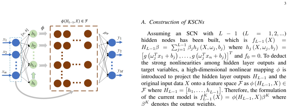
On its own terms, the paper discovers that the SCN supervisory mechanism can be carried into a kernelized model. The KSCN output is $f^K_L = K(K+\tau I)^{-1}Y$, where $K$ is the Gaussian kernel evaluated on the concatenation of SCN hidden activations and original inputs. Theorem 1 states that if each added node satisfies $\langle e^K_{L-1,m}, h_L\rangle^2 \ge b_h^2\delta^K_L$ and output weights are obtained from (7), then $\lim_{L\to\infty}\|f - f^K_L\| = 0$. The proof obtains this by bounding the KSCN error by the standard SCN error, using a decomposition in which the identity mapping is a particular case of the nonlinear feature map. The paper further argues through eigenvalue plots that supervised bases produce a more concentrated Gram-matrix spectrum, which it identifies as favorable for regression.

Load-bearing premise

The proof assumes the KSCN prediction splits into an SCN part and a kernel-only part, with the SCN part obeying the standard error-reduction inequality; if that split fails for the chosen kernel, the convergence guarantee is unsupported.

Editorial extensions

If this is right

KSCNs trained with early stopping need fewer hidden nodes than SCNs to reach comparable accuracy on the tested problems, reducing model size and computational cost.
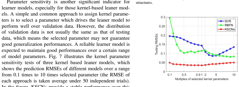
KSCN predictions stay nearly flat when the kernel parameter varies from 0.1 times to 10 times the selected value, while SVR and RBFN degrade substantially.
Across 50 independent trials, KSCN RMSE has smaller standard deviation than SCN, RVFL, MLP, and RBFN on all three datasets, indicating greater performance stability for a randomized learner.
The universal approximation guarantee transfers to the kernelized model, so the residual norm decreases monotonically and tends to zero as supervised nodes are added.

Reading between the lines

Editorial extensions of the paper, not claims the author makes directly.

The decomposition asserted in Equation (15) may restrict which kernels admit the proof; testing non-Gaussian kernels would reveal whether the convergence guarantee is kernel-specific or holds for any Mercer kernel.
The eigenvalue-concentration argument suggests a practical model-selection criterion: prefer kernel parameters and node configurations that concentrate the Gram-matrix spectrum, but the paper does not turn this into an explicit algorithm.
The comparison with kernel RVFL indicates that the supervisory mechanism, not kernelization alone, drives the performance gain; ablating supervision while keeping the same kernel would make the dependence testable.
Because the paper shows sensitivity to the regularization factor, the practical recipe is to pair-search it with the kernel parameter rather than tune either in isolation.

Share X Bluesky LinkedIn Reddit HN

Editorial analysis

A structured set of objections, weighed in public.

Desk editor's note, referee report, and a circularity audit.

Desk Editor's Note

read the letter

Colleague,

Read the KSCN paper. The genuinely new thing is the kernel construction: use SCN's supervised random bases plus raw inputs as the argument of a Gaussian kernel, then solve kernel ridge regression. That is a direct combination of SCN and kernel RVFL, but I don't see it in their cited references, so it's new and incremental. The experiments back the practical claim. On all three datasets KSCN beats SCN and the other baselines in RMSE, and the variance across 50 trials is much smaller. The comparisons against KRVFL and the early-stopping/parameter-sensitivity tables are useful and honestly presented. The eigenvalue-distribution motivation is suggestive rather than rigorous, but it is clearly labeled as an illustration.

The soft spot is Theorem 1. The proof imports the SCN argument by writing the new estimator as the old one plus a correction along the new node h_L. That only works if adding a node appends one feature and leaves the others fixed. But with the Gaussian kernel in Eq. (9), the kernel is computed on [H_L(i), x_i]; when h_L is added, H_L changes for every row, so every entry of the Gram matrix changes. The new predictor is not the old predictor plus a rank-one term, and the chain in Eqs. (15)-(16) doesn't follow. The decomposition f^K_L = sum beta^l h + sum phi beta^nl is asserted, not derived, and the phrase "identity-mapping is the specific form of nonlinear mapping phi" contradicts the Gaussian kernel actually used. On top of that, f^K_L is a ridge estimate with fixed tau; even if the decomposition held, positive tau leaves a residual that won't vanish as L grows. The proof would need tau depending on L and going to zero, plus a node-selection inequality adapted to kernel ridge regression. None of that is there.

So the empirical method is plausible and the UAP claim is not. This is the central gap. I'd also note minor stuff: the proof has typos (e^*_L vs e^K_L, subscripts m vs q), and no code or data for the industrial datasets is provided, which makes the empirical claims harder to check.

Who is this for? People working on randomized neural networks, SCN variants, and soft sensors. They get a reasonable empirical recipe and a clear question to fix. The paper deserves a serious referee, but the referee should require either a corrected convergence proof with tau_L -> 0, or a downgrade of the theoretical claim to a conjecture/observation. I would not desk-reject it.

Recommendation: send to review, with the theory as the main condition.

Referee Report

3 major / 5 minor

Summary. The paper proposes kernel stochastic configuration networks (KSCNs), in which the hidden-node outputs of an SCN are concatenated with the raw inputs and mapped through a Gaussian kernel; the output weights are obtained from the regularized least-squares solution f^K_L = K(K + τI)^{-1}Y. The authors claim that KSCNs inherit the universal approximation property of SCNs, justify the construction via an eigenvalue-distribution argument, and report experiments on one synthetic and two industrial regression problems showing lower RMSE and higher stability than SCNs, SVR, RBFN, RVFL, and MLP. The empirical results are plausible and the paper is clearly written, but the theoretical convergence proof contains a load-bearing unsupported decomposition and an invalid application of the SCN error-reduction argument to a regularized kernel estimator.

Significance. If the universal approximation claim were established, KSCNs would be a useful contribution to randomized neural-network regression, combining SCN's supervisory node allocation with kernel-based representation learning. The experimental study is a genuine strength: it reports 50-trial comparisons with detailed RMSE, R^2, early-stopping behavior, kernel-parameter sensitivity, and comparisons against kernel RVFL, and it includes two real industrial datasets. However, the paper's central theoretical assertion is currently unsupported, and because the abstract and Section III-B both place weight on this claim, the contribution is only partially substantiated.

major comments (3)

[Section III-B, Eq. (15)] The proof of Theorem 1 assumes the decomposition f^K_L = Σ_{j=1}^L β^l_j h_j + Σ_{j=1}^{D-L} φ_j(H_L,X) β^nl_j, but this is asserted without derivation. In the construction, f^K_L = K(K+τI)^{-1}Y with the Gaussian kernel of Eq. (9), and there is no argument showing that this estimator lies in the sum of the span of the individual hidden-node vectors h_j and an additional component of the stated form. The sentence 'Since the identity-mapping is the specific form of nonlinear mapping φ' does not establish the decomposition for the Gaussian kernel actually used in the experiments, and the inequality in Eq. (15) therefore does not follow.
[Section III-B, Eq. (16)] The residual update e^K_L = e^K_{L-1} - φ_L(h_L,X)β^K_L presupposes that adding hidden node L appends one new feature while all previous features remain unchanged. In the actual kernel construction (Eq. (9)), adding h_L changes the concatenated vector [H_L(i), x_i^T] for every sample i, so every entry of the kernel Gram matrix K changes globally. The new estimator is not the old estimator plus a rank-one correction along h_L, so the chain of inequalities imported from the SCN proof in [7]—which relies on such an additive update—does not apply.
[Section III-B, Theorem 1 and Eq. (10)] Even if the decomposition in Eq. (15) were granted, f^K_L is a ridge-regularized estimator with fixed τ > 0. The SCN convergence theorem in [7] applies to the unregularized least-squares projection onto the hidden-node span. For a fixed positive τ, the regularized estimate retains a bias term that does not vanish as L → ∞, so the conclusion lim_{L→∞} ||f - f^K_L|| = 0 requires either τ_L → 0 or an explicit bound on the regularization bias; neither is stated or used. Because Theorem 1 is the basis of the universal-approximation claim, this gap is load-bearing.

minor comments (5)

[Section III-B, Eq. (13)] The subscript in δ^K_{L,q} is inconsistent: Eq. (13) defines δ^K_{L,q} = (1 - r - μ_L) ||e^K_{L-1,m}||^2 using m, while Eq. (14) and the proof use m and q interchangeably. Please unify the index notation.
[Section III-B, Eq. (16)] The denominator in the final inequality is written b^2_n in one place and b^2_h in another; these should be the same symbol, presumably b^2_h from Eq. (14).
[Section III-D, Algorithm 1] The text states that the detailed procedures are demonstrated in Algorithm 1, but the algorithm block is not present in the manuscript. Either include the pseudocode or remove the reference.
[Section IV-B, Fig. 9] Figure 9 compares RVFL, SCNs, KRVFL, and KSCNs, but KRVFL is not introduced in the main model list; the definition and parameter settings of KRVFL appear only later, in the discussion of Fig. 11. Please define KRVFL earlier or in the figure caption.
[Section IV-D, Table VII] The text says 'the value of regularization factor is pair-searched along with the kernel parameter,' but the tables report RMSEs for fixed kernel parameters while varying τ; this is a minor wording issue, as the two-parameter search is described elsewhere.

Circularity Check

2 steps flagged · score 4.0 of 10

Theorem 1's universal-approximation claim asserts an identity feature map to inherit convergence from the authors' SCN theorem, while the implemented Gaussian kernel (Eq. 9) is not identity; the central theoretical claim is a reduction, not a derivation.

ansatz smuggled in via citation [Section III-B, Theorem 1 proof, Eq. (15)]
"Since the identity-mapping is the specific form of nonlinear mapping φ, it is obvious to obtain ∥eK L∥2 ≤ ∥e∗ L∥2 due to the reason that ∥eK L∥2 =∥f − PL j=1 βl j hj − PD−L j=1 ϕj (HL, X) βnl j ∥2 ≤∥f − PL j=1 β∗ j hj∥2 = ∥e∗ L∥2."

This is the only bridge that imports the SCN convergence theorem [7] into KSCNs. It assumes the nonlinear feature map φ contains the identity as a special case, so the KSCN estimator is treated as the SCN estimator plus extra terms. But the KSCN kernel in Eq. (9) is a Gaussian RBF on [H_{L-1}(i), x_i]; its Mercer feature map is not the identity, and no derivation of the decomposition f^K_L = Σβ^l_j h_j + Σφ_j β^nl_j is given. The residual bound is therefore asserted, not derived, and the UAP proof reduces to the SCN theorem under a mapping that is not the mapping used in the algorithm.
self citation load bearing [Section III-B, Theorem 1 proof, Eq. (16)]
"With the conclusions of [7] and above, it can be derived that ∥eK L∥2 = ∥eK L−1 − ϕL (HL, X) βK L ∥2 ≤ ∥eK L−1 − β∗ LhL∥2 ≤ ∥eK L−1 − β′ LhL∥2 ≤ ∥eK L−1∥2."

The step assumes adding the L-th node changes only the single new feature φ_L(h_L,X) and leaves the previous features unchanged, exactly as in the SCN proof of [7]. In KSCNs, however, the kernel matrix (9) is built from all concatenated rows [H_{L-1}(i), x_i]; adjoining h_L changes H_L(i) for every sample, so every entry of K and every feature φ(H_L,X) changes. The new estimator K(K+τI)^{-1}Y is not the old estimator plus a rank-one update along h_L. Thus the chain that inherits convergence from [7] is not the KSCN construction but an SCN-like additive model.

full rationale

Most of the empirical content is non-circular: KSCN is implemented as kernel ridge regression on SCN-generated random bases, hyperparameters are chosen on validation data, and RMSE and R² are reported on held-out test sets against external baselines (SVR, RBFN, RVFL, MLP, SCN, KRVFL). Those measurements are measured rather than derived from fitted constants. The circularity is concentrated in Theorem 1 (Section III-B). The proof's key inequality (15) is justified by 'identity-mapping is the specific form of nonlinear mapping φ,' which makes the KSCN residual bounded by the plain SCN residual and lets the authors import the convergence proof of their own SCN paper [7]. But the KSCN kernel (9) is a Gaussian RBF on [H_{L-1}(i), x_i]; its feature map is not identity, and adding a node changes every row H_L(i), hence the whole Gram matrix. Therefore f^K_L = K(K+τI)^{-1}Y is not the previous estimator plus a rank-one correction along h_L, so Eqs. (15)-(16) do not follow. The theorem reduces to the SCN result by an asserted mapping, rather than proving convergence for the kernel construction actually used. This is a load-bearing self-reduction, but it does not infect the experimental comparisons, so the overall score is moderate.

Assumptions & free parameters 3 free parameters · 4 assumptions · 1 invented entities

The empirical method depends on fitted hyperparameters, namely kernel width, regularization factor, and early stopping patience. The UAP proof relies on SCN's theorem plus an unproved identity-mapping decomposition. No new physical entity is proposed.

free parameters (3)

Gaussian kernel width c = 1.21 (DB1), 99.91 (DB2), 98.61 (DB3)
Selected by validation search over [10^-2, 10^2]; central to the KSCN kernel matrix, with no theoretical prescription.
Regularization factor tau = 0.0001 (DB1), 0.001 (DB2), 0.1 (DB3)
Selected by validation search over [0.1, 0.01, 0.001, 0.0001]; controls the ridge term in Eq. (7).
Early stopping patience pmax = 5 for main results; varied 1 to 9 in comparisons
Hand-chosen tolerance that affects the final number of hidden nodes and the results in Tables II, IV, and VI.

assumptions (4)

standard math span(Gamma) is dense in L2 and all h in Gamma satisfy 0 < ||h|| < b_h
Inherited from SCN theory [7]; invoked in Theorem 1 to guarantee candidate nodes can reduce error.
standard math The Gaussian kernel defines an RKHS via Mercer's theorem
Used in Section III-A to replace phi phi^T with the kernel matrix K.
ad hoc to paper Identity mapping is a specific form of the nonlinear mapping phi
Used in Eq. (15) to bound the KSCN error by the plain SCN error; not true for the Gaussian kernel used in experiments.
domain assumption SCN universal approximation theorem [7] is accepted as a black box
The KSCN convergence proof reduces to the conclusions of [7] rather than proving the regularized kernel ridge case from scratch.

invented entities (1)

Decomposition terms beta^l_j h_j and phi_j(H_L, X) beta^nl_j with implicit dimension D
purpose: Used to express f^K_L as an SCN linear expansion plus extra high-dimensional terms, enabling the UAP proof.
These terms and D are introduced in Eq. (15) without definition or derivation; they do not appear in the model definition Eq. (10).

how reviews work

0 comments

Cite this review

Pith. "Pith review of Kernel Stochastic Configuration Networks for Nonlinear Regression." pith.science (2026). https://pith.science/paper/DTT3HARV

@misc{pith2026241205846,
  author       = {Pith},
  title        = {Pith review of: Kernel Stochastic Configuration Networks for Nonlinear Regression},
  year         = {2026},
  howpublished = {\url{https://pith.science/paper/DTT3HARV}},
  note         = {Machine review of arXiv:2412.05846}
}

read the original abstract

Stochastic configuration networks (SCNs), as a class of randomized learner models, are featured by its way of random parameters assignment in the light of a supervisory mechanism, resulting in the universal approximation property at algorithmic level. This paper presents a kernel version of SCNs, termed KSCNs, aiming to enhance model's representation learning capability and performance stability. The random bases of a built SCN model can be used to span a reproducing kernel Hilbert space (RKHS), followed by our proposed algorithm for constructing KSCNs. It is shown that the data distribution in the reconstructive space is favorable for regression solving and the proposed KSCN learner models hold the universal approximation property. Three benchmark datasets including two industrial datasets are used in this study for performance evaluation. Experimental results with comparisons against existing solutions clearly demonstrate that the proposed KSCN remarkably outperforms the original SCNs and some typical kernel methods for resolving nonlinear regression problems in terms of the learning performance, the model's stability and robustness with respect to the kernel parameter settings.

Figures

Figures reproduced from arXiv: 2412.05846 by the authors.

**Figure 2.** The schematic of SCNs. features about these approaches is the powerful nonlinear expression ability in regression tasks. However, the vast majority of the existing kernel-based learner models, including SVR and RBFN, seeks to project the original data onto a feature space for tackling nonlinearities. The effectiveness of this operation greatly depends on the specific form of the kernel function, which defines a uni… view at source ↗

**Figure 3.** The schematic of KSCNs. of two variables satisfying the Mercer theorem [17], which can define a Hilbert space H. If a kernel K(x, y) has the following property: f (y) = ⟨f (x), K (x, y)⟩H , ∀f ∈ H (3) where ⟨., .⟩H denotes the dot product in H, then K(x, y) is defined as a reproducing kernel for H and H is accordingly called a reproducing kernel Hilbert space. According to Mercer’s theorem, the reproducing kernel K(… view at source ↗

Figures from the paper (11 more)

**Figure 4.** Figure 4: An illustration about how different distributions of Gram matrices’ eigenvalues affect the regression performances. [PITH_FULL_IMAGE:figures/full_fig_p006_4.png]

**Figure 5.** Figure 5: The distributions of eigenvalues of different kernel Gram matrices. [PITH_FULL_IMAGE:figures/full_fig_p006_5.png]

**Figure 6.** Figure 6: Validation processes with early stopping for configuring the hidden [PITH_FULL_IMAGE:figures/full_fig_p007_6.png]

**Figure 7.** Figure 7: Different models’ robustness tests with respect to kernel parameter [PITH_FULL_IMAGE:figures/full_fig_p007_7.png]

**Figure 8.** Figure 8: Basic flowchart of the debutanizer column. [PITH_FULL_IMAGE:figures/full_fig_p007_8.png]

**Figure 9.** Figure 9: Detailed prediction results of (a) RVFL, (b) SCNs, (c)KRVFL and (d) KSCNs. [PITH_FULL_IMAGE:figures/full_fig_p008_9.png]

**Figure 10.** Figure 10: Performance stability tests of different randomized learner models. [PITH_FULL_IMAGE:figures/full_fig_p009_10.png]

**Figure 11.** Figure 11: Performance comparison of KRVFL and KSCNs under different [PITH_FULL_IMAGE:figures/full_fig_p009_11.png]

**Figure 12.** Figure 12: Different models’ robustness tests with respect to kernel parameter [PITH_FULL_IMAGE:figures/full_fig_p009_12.png]

**Figure 13.** Figure 13: Performance stability tests of different randomized learner models. [PITH_FULL_IMAGE:figures/full_fig_p011_13.png]

**Figure 14.** Figure 14: Performance comparison of KRVFL and KSCNs under different [PITH_FULL_IMAGE:figures/full_fig_p011_14.png]

Discussion (0). Continue with ORCID to comment.

Reference graph

Works this paper leans on

35 extracted references · 34 canonical work pages

[7]

Stochastic configuration networks: Fundamentals and algorithms,

D. Wang and M. Li, “Stochastic configuration networks: Fundamentals and algorithms,” IEEE Transactions on Cybernetics , vol. 47, no. 10, pp. 3466–3479, Oct. 2017

work page 2017
[1]

Explaining deep neural networks and beyond: A review of methods and applications,

W. Samek, G. Montavon, S. Lapuschkin, C. J. Anders, and K.-R. Muller, “Explaining deep neural networks and beyond: A review of methods and applications,” Proceedings of the IEEE , vol. 109, no. 3, pp. 247–278, Mar. 2021

work page 2021
[2]

Learning internal representations by back-propagating errors,

D. E. Rumelhart, G. E. Hinton, and R. J. Williams, “Learning internal representations by back-propagating errors,” Nature, vol. 323, no. 6088, pp. 533–536, 1986

work page 1986
[3]

Effective data mining using neural networks,

H. Lu, R. Setiono, and H. Liu, “Effective data mining using neural networks,” IEEE Transactions on Knowledge and Data Engineering , vol. 8, no. 6, pp. 957–961, Dec. 1996

work page 1996
[4]

Editorial: Randomized algorithms for training neural net- works,

D. Wang, “Editorial: Randomized algorithms for training neural net- works,” Information Sciences, vols. 364–365, pp. 126–128, Oct. 2016

work page 2016
[5]

Randomness in neural networks: An overview,

S. Scardapane and D. Wang, “Randomness in neural networks: An overview,” Wiley Interdisciplinary Reviews-Data Mining and Knowledge Discovery, vol. 7, no. 2, pp. 1-18, Apr. 2017

work page 2017
[6]

Insights into randomized algorithms for neural networks: Practical issues and common pitfalls,

M. Li and D. Wang, “Insights into randomized algorithms for neural networks: Practical issues and common pitfalls,” Information Sciences , vols. 382–383, pp. 170–178, Mar. 2017

work page 2017
[8]

Predicting particle size of copper ore grinding with stochastic configuration networks,

D. Wang, P. Tian, W. Dai, and G. Yu, “Predicting particle size of copper ore grinding with stochastic configuration networks,” IEEE Transactions on Industrial Informatics , vol. 20, no. 11, pp. 12969-12978, Nov. 2024

work page 2024

Show all 35 references

[9]

2-D stochastic configuration networks for image data analytics,

M. Li and D. Wang, “2-D stochastic configuration networks for image data analytics,” IEEE Transactions on Cybernetics , vol. 51, no. 1, pp. 359–372, Jan. 2021

2021
[10]

Recurrent stochastic configuration networks for temporal data analytics,

D. Wang and G. Dang, “Recurrent stochastic configuration networks for temporal data analytics,” arXiv:2406.16959v2, 2024

2024 arXiv
[11]

Fuzzy recurrent stochastic configuration net- works for industrial data analytics,

D. Wang and G. Dang, “Fuzzy recurrent stochastic configuration net- works for industrial data analytics,” arXiv: 2407.11038v2, 2024

2024 arXiv
[12]

Online self-learning stochastic configura- tion networks for nonstationary data stream analysis,

K. Li, J. Qiao, and D. Wang, “Online self-learning stochastic configura- tion networks for nonstationary data stream analysis,” IEEE Transactions on Industrial Informatics , vol. 20, no. 3, pp. 3222–3231, Mar. 2024

2024
[13]

Fuzzy stochastic configuration networks for nonlinear system modeling,

K. Li, J. Qiao, and D. Wang, “Fuzzy stochastic configuration networks for nonlinear system modeling,” IEEE Transactions on Fuzzy Systems , vol. 32, no. 3, pp. 948-957, Mar. 2024

2024
[14]

Mixed-distribution-based robust stochastic configu- ration networks for prediction interval construction,

J. Lu and J. Ding, “Mixed-distribution-based robust stochastic configu- ration networks for prediction interval construction,” IEEE Transactions on Industrial Informatics , vol. 16, no. 8, pp. 5099–5109, Aug. 2020

2020
[15]

Ensemble stochastic configuration networks for estimating prediction intervals: A simultaneous robust train- ing algorithm and its application,

J. Lu, J. Ding, X. Dai, and T. Chai, “Ensemble stochastic configuration networks for estimating prediction intervals: A simultaneous robust train- ing algorithm and its application,” IEEE Transactions on Neural Networks and Learning Systems , vol. 31, no. 12, pp. 5426–5440, Dec. 2020

2020
[16]

Hybrid parallel stochastic configuration networks for industrial data analytics,

W. Dai, X. Zhou, D. Li, S. Zhu, and X. Wang, “Hybrid parallel stochastic configuration networks for industrial data analytics,” IEEE Transactions on Industrial Informatics , vol. 18, no. 4, pp. 2331-2341, Apr. 2022

2022
[17]

Nonlinear component analysis as a kernel eigenvalue problem,

B. Sch ¨olkopf, A. Smola, and K.-R. M ¨uller, “Nonlinear component analysis as a kernel eigenvalue problem,” Neural Computation, vol. 10, no. 5, pp. 1299–1319, Jul. 1998

1998
[18]

Sch ¨olkopf and A.J

B. Sch ¨olkopf and A.J. Smola, Learning with Kernels , Cambridge, MA, USA: MIT Press, 2002

2002
[19]

An introduction to kernel-based learning algorithms,

K.-R. M ¨uller, S. Mika, G. R ¨atsch, K. Tsuda, and B. Sch ¨olkopf, “An introduction to kernel-based learning algorithms,” IEEE Transactions on Neural Networks, vol. 12, no. 2, pp. 181–201, Mar. 2001

2001
[20]

Sup- port vector machines,

M. A. Hearst, S. T. Dumais, E. Osuna, J. Platt, and B. Scholkopf, “Sup- port vector machines,” IEEE Intelligent Systems and their Applications , vol. 13, no. 4, pp. 18–28, Jul. 1998

1998
[21]

A tutorial on support vector regression,

A. J. Smola and B. Sch ¨olkopf, “A tutorial on support vector regression,” Statistics and Computing , vol. 14, no. 3, pp. 199–222, Aug. 2004

2004
[22]

Universal approximation using radial-basis- function networks,

J. Park and I. W. Sandberg, “Universal approximation using radial-basis- function networks,” Neural Computation, vol. 3, no. 2, pp. 246–257, Jun. 1991

1991
[23]

Functional-link net computing: Theory, system architecture, and functionalities,

Y .-H. Pao and Y . Takefuji, “Functional-link net computing: Theory, system architecture, and functionalities,” Computer, vol. 25, no. 5, pp. 76–79, May 1992

1992
[24]

Automatic early stopping using cross validation: Quanti- fying the criteria,

L. Prechelt, “Automatic early stopping using cross validation: Quanti- fying the criteria,” Neural Networks , vol. 11, no. 4, pp. 761–767, Jun. 1998

1998
[25]

Principal composite kernel feature analysis: Data-dependent kernel approach,

Y . Motai and H. Yoshida, “Principal composite kernel feature analysis: Data-dependent kernel approach,” IEEE Transactions on Knowledge and Data Engineering, vol. 25, no. 8, pp. 1863–1875, Aug. 2013

2013
[26]

Feasibility of random basis function approximators for modeling and control,

I. Y . Tyukin and D. V . Prokhorov, “Feasibility of random basis function approximators for modeling and control,” in Proceedings of 2009 IEEE International Conference on Control Applications, St. Petersburg, Russia, Jul. 2009, pp. 1391–1396

2009
[27]

Fortuna, S

L. Fortuna, S. Graziani, A. Rizzo, and M. G. Xibilia, Soft Sensors for Monitoring and Control of Industrial Processes , London, U.K.: Springer, 2007

2007
[28]

A review on soft sensors for monitoring, control, and optimization of industrial processes,

Y . Jiang, S. Yin, J. Dong, and O. Kaynak, “A review on soft sensors for monitoring, control, and optimization of industrial processes,” IEEE Sensors Journal, vol. 21, no. 11, pp. 12868-12881, Jun. 2021

2021
[29]

Variational inference over graph: Knowl- edge representation for deep process data analytics,

Z. Chen, Z. Song, and Z. Ge, “Variational inference over graph: Knowl- edge representation for deep process data analytics,” IEEE Transactions on Knowledge and Data Engineering , vol. 36, no. 6, pp. 2730–2744, Jun. 2024

2024
[30]

Transfer learning for dynamic fea- ture extraction using variational bayesian inference,

J. Xie, B. Huang, and S. Dubljevic, “Transfer learning for dynamic fea- ture extraction using variational bayesian inference,” IEEE Transactions on Knowledge and Data Engineering , vol. 34, no. 11, pp. 5524–5535, Nov. 2022

2022
[31]

Multi-label classifier based on kernel random vector functional link network,

V . Chauhan, A. Tiwari, and S. Arya, “Multi-label classifier based on kernel random vector functional link network,” in Proceedings of 2020 International Joint Conference on Neural Networks , Glasgow, United Kingdom: IEEE, Jul. 2020, pp. 1–7

2020
[32]

Kernel-based random vector functional-link network for fast learning of spatiotemporal dynamic processes,

K.-K. Xu, H.-X. Li, and H.-D. Yang, “Kernel-based random vector functional-link network for fast learning of spatiotemporal dynamic processes,” IEEE Transactions on Systems Man Cybernetics-Systems, vol. 49, no. 5, pp. 1016–1026, May 2019

2019
[33]

A comprehensive survey on regularization strategies in machine learning,

Y . Tian and Y . Zhang, “A comprehensive survey on regularization strategies in machine learning,” Information Fusion, vol. 80, pp. 146–166, Apr. 2022

2022
[34]

Stochastic configuration machines for industrial artificial intelligence,

D. Wang and M. J. Felicetti, “Stochastic configuration machines for industrial artificial intelligence,” arXiv:2308.13570v6, 2023

2023 arXiv
[35]

Stochastic configuration machines: FPGA implementation,

M. J. Felicetti and D. Wang, “Stochastic configuration machines: FPGA implementation,” arXiv: 2310.19225v1, 2024

2024 arXiv

Pith tools

Reviewed August 11, 2026 · model on record in the stance chip above.

[1] [7]

Stochastic configuration networks: Fundamentals and algorithms,

D. Wang and M. Li, “Stochastic configuration networks: Fundamentals and algorithms,” IEEE Transactions on Cybernetics , vol. 47, no. 10, pp. 3466–3479, Oct. 2017

work page 2017

[2] [1]

Explaining deep neural networks and beyond: A review of methods and applications,

W. Samek, G. Montavon, S. Lapuschkin, C. J. Anders, and K.-R. Muller, “Explaining deep neural networks and beyond: A review of methods and applications,” Proceedings of the IEEE , vol. 109, no. 3, pp. 247–278, Mar. 2021

work page 2021

[3] [2]

Learning internal representations by back-propagating errors,

D. E. Rumelhart, G. E. Hinton, and R. J. Williams, “Learning internal representations by back-propagating errors,” Nature, vol. 323, no. 6088, pp. 533–536, 1986

work page 1986

[4] [3]

Effective data mining using neural networks,

H. Lu, R. Setiono, and H. Liu, “Effective data mining using neural networks,” IEEE Transactions on Knowledge and Data Engineering , vol. 8, no. 6, pp. 957–961, Dec. 1996

work page 1996

[5] [4]

Editorial: Randomized algorithms for training neural net- works,

D. Wang, “Editorial: Randomized algorithms for training neural net- works,” Information Sciences, vols. 364–365, pp. 126–128, Oct. 2016

work page 2016

[6] [5]

Randomness in neural networks: An overview,

S. Scardapane and D. Wang, “Randomness in neural networks: An overview,” Wiley Interdisciplinary Reviews-Data Mining and Knowledge Discovery, vol. 7, no. 2, pp. 1-18, Apr. 2017

work page 2017

[7] [6]

Insights into randomized algorithms for neural networks: Practical issues and common pitfalls,

M. Li and D. Wang, “Insights into randomized algorithms for neural networks: Practical issues and common pitfalls,” Information Sciences , vols. 382–383, pp. 170–178, Mar. 2017

work page 2017

[8] [8]

Predicting particle size of copper ore grinding with stochastic configuration networks,

D. Wang, P. Tian, W. Dai, and G. Yu, “Predicting particle size of copper ore grinding with stochastic configuration networks,” IEEE Transactions on Industrial Informatics , vol. 20, no. 11, pp. 12969-12978, Nov. 2024

work page 2024