Tensor-based computation of metastable and coherent sets

Cecilia Clementi; Feliks N\"uske; Patrick Gel{\ss}; Stefan Klus

REVIEW 3 major objections 4 minor 52 references

Tensor-based computation of metastable and coherent sets

T0 review · 3 major / 4 minor · reviewed 2026-08-14 · deepseek-v4-flash

Challenge this review Re-run · record.json Download PDF Read on arXiv ↗ Review JSON

Pith's one-line read Tensor-train decompositions let EDMD and CCA run on high-dimensional data without forming the full basis matrix.

desk verdict A practical and mostly sound tensor-train EDMD/CCA paper with impressive molecular benchmarks; the convergence proof has a fixable max-vs-min spectral gap slip that should be corrected. read the letter →

arxiv 1908.04741 v3 pith:DUJGA4B4 submitted 2019-08-12 math.NA cs.LGcs.NAmath.DSphysics.comp-phstat.ML

Feliks Nüske , Patrick Gel{ss} , Stefan Klus , Cecilia Clementi This is my paper · ORCID

classification math.NAcs.LGcs.NAmath.DSphysics.comp-phstat.ML MSC 15A6937L6537M1062H2092C40

keywords Koopmanoperatorextendeddynamicmodedecompositiontensortrainformatcanonicalcorrelationanalysiscoherentsetsmetastabledynamicshigh-dimensionalsystemsforward-backward

verification ladder T0 review T1 audit T2 compute T3 formal

The pith

A machine-rendered reading of the paper's core claim, the machinery that carries it, and where it could break.

The reading

Koopman-based analysis of dynamical systems is usually limited by the cost of building and diagonalizing large matrices of basis-function evaluations. This paper removes that bottleneck for tensor-product basis sets by storing the data tensor, the evaluations of all product basis functions at all snapshots, in the tensor-train (TT) format, and deriving tensor-based versions of the EDMD and canonical correlation analysis algorithms. The key claim is that these tensor algorithms, AMUSEt for EDMD and tensor CCA for coherent sets, yield a reduced matrix eigenvalue problem with the same spectrum as the full problem on a fixed-rank subspace, and that this subspace converges to a deterministic Galerkin subspace as the number of snapshots grows. If correct, this makes slow metastable dynamics and coherent sets computable for high-dimensional systems with very large basis sets, as the paper demonstrates on peptide simulations and the ABC flow.

What carries the argument

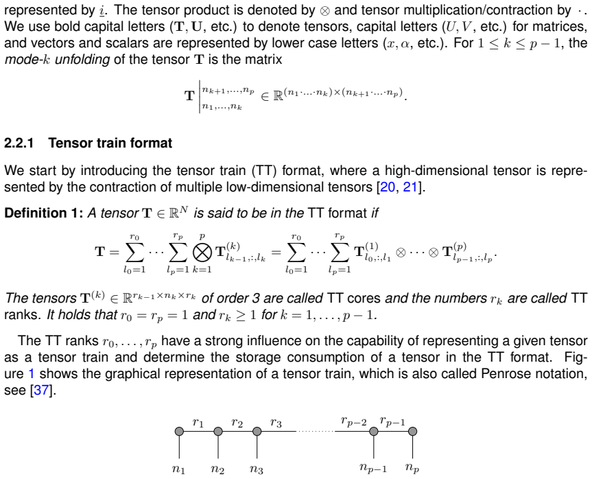
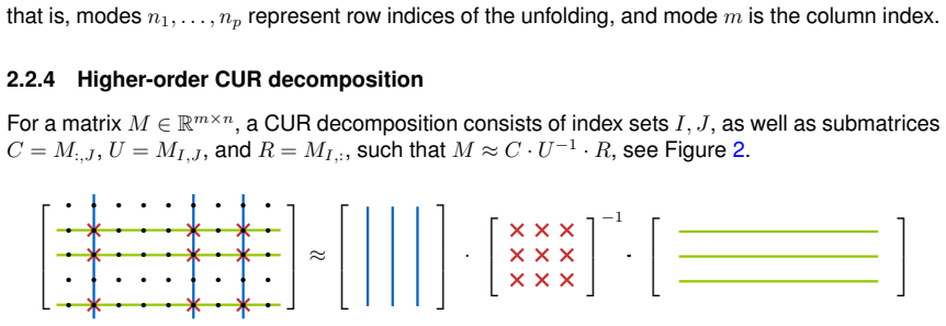
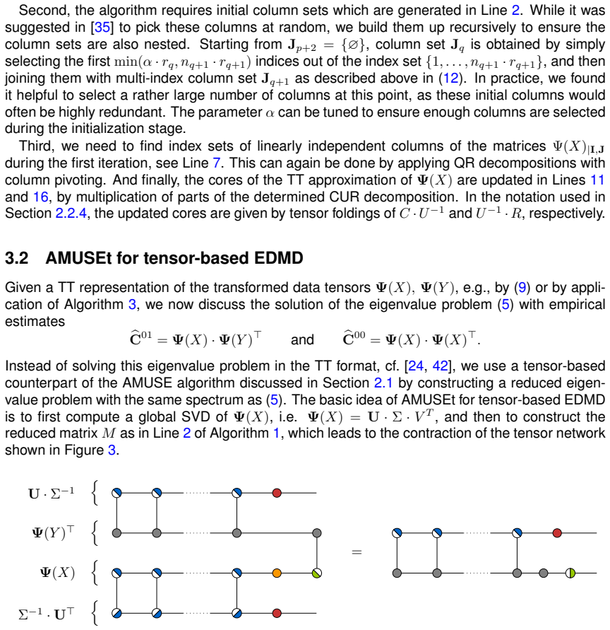
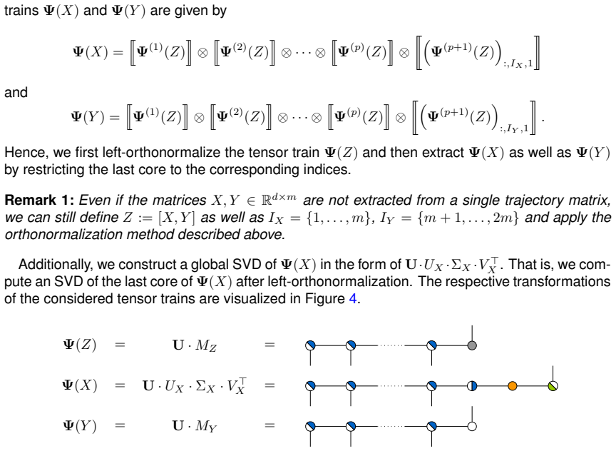
The central object is the transformed data tensor $\Psi(X)$, an order-$(p+1)$ tensor formed by evaluating every product basis function $\psi_1(x_k)\otimes\cdots\otimes\psi_p(x_k)$ at every snapshot and appending the snapshot index. Its TT decomposition represents this tensor as a chain of small cores with linking ranks $r_k$, a low-parameter representation of a high-dimensional array. AMUSEt uses a global SVD of the TT tensor, namely a segment $U$, a diagonal matrix $\Sigma$, and an orthonormal $V$, to build the reduced matrix $M$; orthonormality of the cores makes almost all contractions cancel, so only the final cores and $\Sigma^{-1}$ enter. The paper also introduces HOCUR, a greedy higher-order CUR decomposition of $\Psi(X)$ based on maximum-volume index selection, which avoids building the full tensor. The convergence argument is carried by the recursive subspaces $F_k$, obtained by compressing $U_k=F_{k-1}\otimes V_k$ to its leading $r_k$ eigenvectors, and by Davis-Kahan type perturbation estimates showing that the distance $d(F_k,\hat{F}_k)$ shrinks as more data are used.

What would settle it

Take a system for which the exact TT ranks of $\Psi(X)$ at a fixed accuracy are known to be large, such as a tensor-product basis on strongly interacting coordinates with no low-rank structure, compute AMUSEt with a deliberately small rank cap, and compare the slowest eigenvalues against a dense EDMD solution on the same data; if the reduced spectrum diverges while dense EDMD is still feasible, the rank assumption underlying the method's efficiency is violated and the advantage over dense EDMD disappears as the ranks grow.

Watch

Extended reading notes

Core claim

The paper's central claim is that for a tensor-product trial space, EDMD and forward-backward/CCA analysis can be carried out on a low-rank tensor-train representation of the transformed data tensor $\Psi(X)=\sum_{k}\psi_1(x_k)\otimes\cdots\otimes\psi_p(x_k)\otimes e_k$, without ever forming the full Galerkin matrices $C_{00}, C_{01}, C_{10}, C_{11}$. The tensor algorithm AMUSEt first computes a global SVD of $\Psi(X)$ in TT form; because the TT cores are orthonormal, the reduced matrix $M=V_X^{\top}M_Y^{\top}U_X\Sigma_X^{-1}$ contains the same spectrum as the standard EDMD eigenproblem on the subspace spanned by the left singular vectors. Analogously, tensor CCA constructs a reduced matrix from separate global SVDs of $\Psi(X)$ and $\Psi(Y)$, yielding eigenfunctions of the forward-backward operator and hence coherent sets. The paper proves that, under ergodicity and a singular-value gap assumption, the data-driven subspace converges to a deterministic fixed subspace $F_p$ in the infinite-data limit, so that AMUSEt converges to a Galerkin approximation of the Koopman or forward-backward operator on that subspace.

Load-bearing premise

The method's speed and memory advantage rests on the transformed data tensor admitting a small tensor-train rank, and on the greedy HOCUR iteration actually finding that small-rank representation; when that fails, the reduced eigenvalue problem no longer captures the dynamics of interest.

Editorial extensions

If this is right

Users can apply AMUSEt to a tensor-product basis with very many basis functions without storing the full Galerkin matrices, since the reduced matrix never exceeds the number of snapshots.
For reversible systems the resulting slowest implied timescales respect the variational principle, so smaller truncation thresholds select larger subspaces and give closer approximations.
For non-reversible or time-dependent dynamics, tensor CCA extracts finite-time coherent sets directly from trajectory data, as demonstrated on the ABC flow.
In the infinite-data limit the method is a Galerkin approximation of the Koopman or forward-backward operator on the deterministic subspace $F_p$, giving the procedure a physical interpretation.
The HOCUR variant can process data sets and basis sizes that are intractable for direct construction, as shown on a high-dimensional protein data set with millions of frames.

Reading between the lines

Editorial extensions of the paper, not claims the author makes directly.

An implicit consequence is that the fixed-rank subspace $F_p$ could serve as a built-in feature-selection or coarse-graining layer: the algorithm decides which products of univariate functions matter, making it a data-driven alternative to hand-crafted collective variables.
A natural testable extension is to use the AMUSEt spectrum as a cheap surrogate during basis construction, adaptively adding univariate functions while monitoring whether the slowest timescales change and avoiding a full refit.
Because the convergence proof is stated for the exact TT decomposition, extending it to bound the error introduced by the greedy HOCUR approximation would be a direct next step; until then, practical users may need residual-based rank-adaptivity or stopping criteria.
If TT ranks turn out to be large for strongly coupled variables, combining HOCUR with nonlinear feature maps or kernel evaluations is a plausible route, and the subspace interpretation would likely carry over.

Share X Bluesky LinkedIn Reddit HN

Signed reviews

No signed human review yet.

Editorial analysis

A structured set of objections, weighed in public.

Desk editor's note, referee report, and a circularity audit.

Desk Editor's Note

read the letter

Bottom line: the paper is worth reading and mostly earns its claims. It scales EDMD and coherent-set CCA to tensor product bases far beyond dense matrix limits, and the NTL9 demonstration with a 3^20 basis and about 1.4 million frames is the right kind of stress test. The main thing to know before citing the convergence result: Proposition 1 has a max-vs-min spectral gap slip, so as printed the infinite-data corollary is not proven.

What is new: AMUSEt for EDMD, the tensorized CCA variant, and the HOCUR construction for transformed data tensors are not restatements of [31,32,34]. The reduction in Eq. (13) is clean, and Lemma 2 gives the right subspace interpretation. The benchmarks compare against external MSM references; the timescales and contact maps line up. That is real evidence the method works at scale. The ABC flow example is more of a sanity check, but fine.

The soft spot is the convergence analysis. The stress-test note is correct: they define δ := max_k δ_k, while every Davis-Kahan step needs a lower bound on the gap, i.e. δ := min_k δ_k. With max, the error tolerances in Steps 1 and k are too large and the induction does not close. This is almost certainly a one-line typo, not a structural flaw, but Corollary 1 is not established by the printed proof. The abstract's claim that the infinite-data limit is established should be qualified until this is fixed.

Two smaller issues. The theorem covers only the exact decomposition (9) at fixed ranks, while the implementation uses adaptive relative truncation and HOCUR, so the formal result is narrower than the numerical section. HOCUR itself has no convergence or error bound; the method's efficiency depends on unproven low TT-rank of the transformed data tensor. That is a genuine limitation, though honestly framed. Also, the benchmarks have no error bars, so the agreement with references is suggestive rather than quantitative. Minor.

Citation pattern is fine. There is heavy self-citation, but to the building blocks (AMUSE, TT-SVD, CUR, prior tensor EDMD), and the new algorithmic content is distinguishable. The paper is for anyone who wants to use high-dimensional product bases with Koopman or transfer-operator methods, and for tensor numerical linear algebra readers. It deserves a serious referee. Recommendation: send to peer review; ask for the δ fix, a qualified infinite-data claim, and error bars or at least a statement of variability in the experiments.

Referee Report

3 major / 4 minor

Summary. This paper combines tensor-train (TT) decompositions with the AMUSE formulation of extended dynamic mode decomposition (EDMD) and canonical correlation analysis (CCA). It introduces a greedy higher-order CUR (HOCUR) scheme for representing transformed data tensors, derives a reduced matrix eigenvalue problem (Eq. (13)) whose spectrum coincides with the EDMD/CCA problem on the selected subspace, proves a subspace interpretation (Lemma 2) and an infinite-data convergence result (Proposition 1, Corollary 1) for the exact TT decomposition, and reports numerical experiments on deca-alanine, NTL9, and ABC flow.

Significance. The derivation is elegant and the algorithmic idea is valuable: for product bases the reduced matrix can be assembled by contracting only a few TT cores, avoiding dense N x N Galerkin matrices. The numerical results are encouraging, showing close agreement with Markov state models and substantial scalability (up to 3^20 basis functions). If the convergence proof is repaired, the paper provides a useful and principled tensor framework for transfer operator approximation. The main current weaknesses are that the central theorem is not proven as printed and the practical HOCUR/adaptive-rank algorithm is not covered by the theory.

major comments (3)

[Section 3.4 / Appendix A (Proposition 1)] In the proof of Proposition 1, the constant is defined as delta := max_k delta_k, where delta_k are the spectral gaps of the matrices C00_U_k. The Davis-Kahan applications in Eqs. (15)-(16) require the inverse of the gap of the specific matrix C00_U_k, i.e. a factor 1/delta_k; with delta = max_k delta_k the coefficient 1/delta is smaller than 1/delta_k, so the stated bounds are not implied. Consequently Eq. (17) and Corollary 1 are not established as written. Replacing delta by min_k delta_k would repair the argument, but the printed proof needs this correction.
[Section 3.4 vs. Sections 3.1-3.2 and 4] Proposition 1 assumes fixed ranks r_k and the exact TT decomposition (9). The numerical method in Section 3.2 and the experiments in Section 4 use adaptive rank truncation with a relative tolerance epsilon (e.g., epsilon = 10^-3 in Figure 6c) and the HOCUR approximation from Algorithm 3, for which no convergence or error bound is provided. Therefore the infinite-data subspace interpretation is not shown for the actually implemented algorithm. The authors should either extend the analysis to these cases or explicitly state that the convergence result applies only to the exact fixed-rank decomposition.
[Section 3.1 (Algorithm 3)] The greedy HOCUR iteration in Algorithm 3 is described as running until convergence, but no convergence criterion, fixed-point property, or error bound is given. Since all large-scale examples in Section 4 rely on HOCUR, the efficiency and accuracy claims rest on an unverified assumption that the iteration produces a small fixed-rank TT approximation. A formal analysis would be preferable; at minimum the authors should state clearly that this is a heuristic and report the observed rank growth or stopping behavior.

minor comments (4)

[Section 3.2, Eq. (13)] In Eq. (13), the symbol U_x should read U_X for consistency with the surrounding notation.
[Section 4.1] The text refers to the 'HOSVD method' although earlier sections call the procedure 'global SVD'; please align the terminology.
[Section 3.1, Algorithm 3] Algorithm 3 does not specify a stopping criterion for the outer loop; please state that the iteration is run for N sweeps and describe which convergence monitor is used.
[Figure 6] The color scale in Figure 6(c) is not explained in the caption; please add the mapping from color to t2 values.

Circularity Check

0 steps flagged · score 0.0 of 10

No circularity found: the AMUSEt reduced matrix is an algebraic identity derived from data SVDs, and the infinite-data limit is proved from independent spectral perturbation arguments.

full rationale

The central derivations are self-contained linear algebra. Equation (13) and the surrounding tensor-network contractions show that the reduced matrix M is obtained by SVD truncation of the data tensors and exact contraction of orthonormal cores; this is a constructive derivation, not a fitted parameter renamed as a prediction. Lemma 1 similarly proves the CCA/forward-backward reduction from the SVD identities. Proposition 1 is a convergence theorem whose hypotheses are singular value gaps of Galerkin matrices and ergodicity of the sampling process, and whose proof uses Davis-Kahan-type perturbation bounds; it does not take the target eigenvalues or timescales as inputs, so Corollary 1 is a genuine consequence rather than a restatement. The paper's references to prior work by the same authors (e.g., [5], [26], [31], [34]) provide standard building blocks such as AMUSE, TT representations, and SVD algorithms, but those works are not used to force the paper's conclusion by invocation of an imported uniqueness theorem, and the present paper re-derives the relevant subspace structure in Lemma 2 and Proposition 1. Numerical validation compares against external MSM, TICA, and flow references ([45], [47], [50]), so the reported timescales and coherent sets are not self-referential. The unproven low-rank assumption underlying HOCUR and the apparent δ = max_k δ_k versus min_k δ_k issue in Appendix A are correctness or robustness concerns, not circularity: they do not make any derived quantity equal to its input by definition.

Assumptions & free parameters 5 free parameters · 4 assumptions · 0 invented entities

The central theory uses standard dynamical systems and perturbation-theory assumptions, with the main practical risk being the low-rank approximability of the data tensor. The numerical results also depend on several hand-chosen basis and truncation parameters; these do not affect the core algebra but are necessary to reproduce the specific benchmark numbers.

free parameters (5)

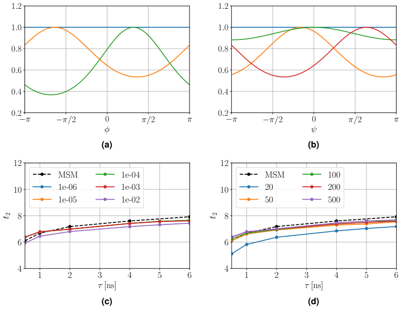
Relative SVD truncation tolerance epsilon = 1e-5, 1e-3, 1e-4, 1e-3 depending on experiment
Controls the rank truncation in the global SVD; affects the size of the reduced matrix and the inferred timescale. Value is chosen by hand for each benchmark.
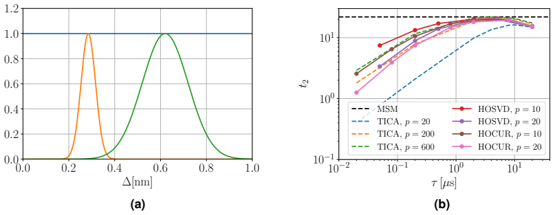
Maximum TT ranks for HOCUR = 50 for deca-alanine, 1000 for NTL9
Hyperparameters bounding the ranks in Algorithm 3; chosen manually, with no automatic selection rule or error bound.
Deca-alanine Gaussian basis parameters = phi: c={-2,1}, s={0.8,0.5}; psi: c={-0.5,0.0,2.0}, s={0.8,4.0,0.8}
Centers and widths are chosen to align with the marginal dihedral distributions of the data, i.e., tuned to the benchmark rather than derived from theory.
NTL9 Gaussian basis parameters = c={0.285,0.62}, s={0.001,0.01}
Centers and widths chosen so that linear combinations of the Gaussians reproduce the distance distributions; effectively fitted to the data.
ABC flow basis parameters = 10 Gaussian functions per dimension with variance 1 on an equidistant grid
Coordinate-major basis chosen by the user for the coherent-set test; no selection criterion is given.

assumptions (4)

domain assumption The stochastic process is ergodic or stationary with an invariant measure so that empirical Gram matrices converge to their analytical counterparts.
Invoked in the proof of Proposition 1, Step 1 and Step k, to bound ||C_hat^00_V1 - C^00_V1||_2. Not stated in the abstract and does not cover time-dependent CCA.
domain assumption For each k, the Galerkin matrices C^00_U_k have a positive singular value gap between the r_k-th and the (r_k+1)-th singular value.
Assumed in Proposition 1; the Davis-Kahan argument collapses without it.
ad hoc to paper The transformed data tensor has an accurate low-TT-rank representation, or the HOCUR iteration converges to one.
Needed for AMUSEt and HOCUR to be more efficient than dense EDMD. No error bounds are provided for the HOCUR approximation, so this is an unproven load-bearing assumption.
domain assumption Basis functions are tensor products of univariate functions and elementary basis evaluations are computable.
The data tensor construction in Eqs. (8)-(9) and the submatrix evaluation formula in Section 3.1 both rely on this product structure.

how reviews work

0 comments

Cite this review

Pith. "Pith review of Tensor-based computation of metastable and coherent sets." pith.science (2026). https://pith.science/paper/DUJGA4B4

@misc{pith2026190804741,
  author       = {Pith},
  title        = {Pith review of: Tensor-based computation of metastable and coherent sets},
  year         = {2026},
  howpublished = {\url{https://pith.science/paper/DUJGA4B4}},
  note         = {Machine review of arXiv:1908.04741}
}

read the original abstract

Recent years have seen rapid advances in the data-driven analysis of dynamical systems based on Koopman operator theory and related approaches. On the other hand, low-rank tensor product approximations -- in particular the tensor train (TT) format -- have become a valuable tool for the solution of large-scale problems in a number of fields. In this work, we combine Koopman-based models and the TT format, enabling their application to high-dimensional problems in conjunction with a rich set of basis functions or features. We derive efficient algorithms to obtain a reduced matrix representation of the system's evolution operator starting from an appropriate low-rank representation of the data. These algorithms can be applied to both stationary and non-stationary systems. We establish the infinite-data limit of these matrix representations, and demonstrate our methods' capabilities using several benchmark data sets.

Figures

Figures reproduced from arXiv: 1908.04741 by the authors.

**Figure 1.** Graphical representation of a tensor train: A core is depicted by a circle with different arms indicating the modes of the tensor and the rank indices. The first and the last TT core are regarded as matrices due to the fact that r0 = rp = 1. We also represent TT cores as two-dimensional arrays containing vectors as elements. For a given tensor train T ∈ R N with cores T(k) ∈ R rk−1×nk×rk , a single core is written a… view at source ↗

**Figure 2.** CUR decomposition: The matrix on the left-hand side is approximated by the matrix product C · U −1 · R, where C (blue lines) is a column subset, R (green lines) is a row subset, and U (red crosses) is the intersection matrix. There are different methods to find optimal sets of rows and columns, cf. [39]. An important subproblem is the following: given a set of column indices J = {j1, . . . , jr} with r ≤ min(m, n) (… view at source ↗

**Figure 3.** Graphical representation of the reduced matrix: Given Ψ(X) (in form of a global SVD) and Ψ(Y ), the reduced matrix M ∈ R r×r is computed by contracting the above tensor network. Half-filled circles in blue depict the cores of U, Σ and Σ −1 are represented by orange and red circles, respectively, and the half-filled circle in green depicts the matrix V of the global SVD. Since we here do not assume any further proper… view at source ↗

Figures from the paper (6 more)

**Figure 4.** Figure 4: Construction of transformed data tensors: The tensor trains Ψ(X) and Ψ(Y ) are extracted from the left-orthonormalized tensor train Ψ(Z). Additionally, Ψ(X) is represented by its global SVD. Again, the cores of U (as well as UX) are represented by half-filled circles …

**Figure 5.** Figure 5: Graphical representation of the eigentensors and eigenfunctions: The tensor train Ξ is built by the contraction of U, UX, Σ −1 , and W (depicted by the square). The matrix Φ comprising the evaluations of the eigenfunctions at the given snapshots is constructed by multi…

**Figure 6.** Figure 6: Results for molecular dynamics simulation data of deca-alanine peptide: (a) Univariate basis set used for all φ-dihedral angles, comprised of the constant and periodic Gaussians centered at cik = {−2, 1}, with sik = {0.8, 0.5}. (b) The same for all ψ-dihedral angles, …

**Figure 7.** Figure 7: Results for molecular dynamics simulation data of NTL9 protein: (a) Univariate basis set used for all distance coordinates, comprised of the constant and Gaussian functions centered at cik = {0.285, 0.62}, with sik = {0.001, 0.01}. (b) Slowest timescale obtained from (…

**Figure 8.** Figure 8: States of NTL9: (a) Contact map for the unfolded state computed from the first two eigenfunctions of the HOCUR model at lag time τ = 5 µs (upper left triangle), compared to the corresponding contact map of the reference MSM (lower right triangle). (b) The same for the …

**Figure 9.** Figure 9: Results for ABC flow: Six coherent vortices in the domain, extracted by applying tCCA. 17 [PITH_FULL_IMAGE:figures/full_fig_p017_9.png]

Discussion (0). Continue with ORCID to comment.

Reference graph

Works this paper leans on

52 extracted references · 19 canonical work pages

[1]

Schütte, A

C. Schütte, A. Fischer, W. Huisinga, and P . Deuﬂhard. A direct approach to conformational dynamics based on hybrid Monte Carlo.Journal of Computational Physics, 151(1):146–168, 1999. doi:10.1006/ jcph.1999.6231

arXiv 1999
[2]

Dellnitz and O

M. Dellnitz and O. Junge. On the approximation of complicated dynamical behavior. SIAM Journal on Numerical Analysis, 36(2):491–515, 1999. doi:10.1137/S0036142996313002

doi:10.1137/s0036142996313002 1999
[3]

C. W. Rowley, I. Mezi ´c, S. Bagheri, P . Schlatter, and D. S. Henningson. Spectral analysis of nonlinear ﬂows. Journal of Fluid Mechanics, 641:115–127, 2009. doi:10.1017/S0022112009992059

doi:10.1017/s0022112009992059 2009
[4]

Budiši ´c, R

M. Budiši ´c, R. Mohr, and I. Mezi ´c. Applied Koopmanism. Chaos: An Interdisciplinary Journal of Non- linear Science, 22(4):047510, 2012. doi:10.1063/1.4772195. 19

doi:10.1063/1.4772195 2012
[5]

S. Klus, F . Nüske, P . Koltai, H. Wu, I. Kevrekidis, C. Schütte, and F . Noé. Data-driven model reduction and transfer operator approximation. Journal of Nonlinear Science , 28(3):985–1010, 2018. doi:10. 1007/s00332-017-9437-7

work page 2018
[6]

M. O. Williams, I. G. Kevrekidis, and C. W. Rowley. A data-driven approximation of the Koopman operator: Extending dynamic mode decomposition. Journal of Nonlinear Science , 25(6):1307–1346,

work page
[7]

S. Klus, P . Koltai, and C. Schütte. On the numerical approximation of the Perron–Frobenius and Koop- man operator. Journal of Computational Dynamics, 3(1):51–79, 2016. doi:10.3934/jcd.2016003

doi:10.3934/jcd.2016003 2016
[8]

Noé and F

F . Noé and F . Nüske. A variational approach to modeling slow processes in stochastic dynamical systems. Multiscale Modeling & Simulation, 11:635–655, 2013. doi:10.1137/110858616

doi:10.1137/110858616 2013

Show all 52 references

[9]

Nüske, B

F . Nüske, B. G. Keller, G. Pérez-Hernández, A. S. J. S. Mey, and F . Noé. Variational approach to molecular kinetics. Journal of Chemical Theory and Computation, 10:1739–1752, 2014. doi:10.1021/ ct4009156

2014
[10]

Froyland, N

G. Froyland, N. Santitissadeekorn, and A. Monahan. Transport in time-dependent dynamical systems: Finite-time coherent sets. Chaos: An Interdisciplinary Journal of Nonlinear Science , 20(4):043116, 2010

2010
[11]

Froyland

G. Froyland. An analytic framework for identifying ﬁnite-time coherent sets in time-dependent dynamical systems. Physica D: Nonlinear Phenomena, 250:1–19, 2013

2013
[12]

D. R. Hardoon, S. Szedmak, and J. Shawe-Taylor. Canonical correlation analysis: An overview with application to learning methods. Neural computation, 16(12):2639–2664, 2004

2004
[13]

S. Klus, B. E. Husic, M. Mollenhauer, and F . Noé. Kernel methods for detecting coherent structures in dynamical data. Chaos, 2019. doi:10.1063/1.5100267

2019 doi
[14]

M. O. Williams, C. W. Rowley, and I. G. Kevrekidis. A kernel-based method for data-driven Koop- man spectral analysis. Journal of Computational Dynamics , 2(2):247–265, 2015. doi:10.3934/jcd. 2015005

2015 doi
[15]

S. Klus, I. Schuster, and K. Muandet. Eigendecompositions of transfer operators in reproducing kernel Hilbert spaces. ArXiv e-prints, 2017. arXiv:1712.01572v2

2017 arXiv
[16]

Mardt, L

A. Mardt, L. Pasquali, H. Wu, and F . Noé. VAMPnets for deep learning of molecular kinetics. Nature communications, 9(1):5, 2018. doi:10.1038/s41467-017-02388-1

2018 doi
[17]

J. D. Carroll and J. J. Chang. Analysis of individual differences in multidimensional scaling via an N-way generalization of ’Eckart-Y oung’ decomposition. Psychometrika, 35(3):283–319, 1970. doi: 10.1007/BF02310791

1970 doi
[18]

L. R. Tucker. The extension of factor analysis to three-dimensional matrices. In H. Gulliksen and N. Frederiksen, editors, Contributions to mathematical psychology, pages 110–127. Holt, Rinehart and Winston, 1964

1964
[19]

Hackbusch and S

W. Hackbusch and S. Kühn. A new scheme for the tensor representation. Journal of Fourier analysis and applications, 15(5):706–722, 2009. doi:10.1007/s00041-009-9094-9

2009 doi
[20]

Oseledets and E

I. Oseledets and E. Tyrtyshnikov. Breaking the curse of dimensionality, or how to use SVD in many dimensions. SIAM Journal on Scientiﬁc Computing, 31(5):3744–3759, 2009. doi:10.1137/090748330

2009 doi
[21]

Oseledets

I. Oseledets. Tensor-train decomposition. SIAM Journal on Scientiﬁc Computing, 33:2295–2317, 2011. doi:10.1137/090752286

2011 doi
[22]

M. H. Beck, A. Jäckle, G. A. Worth, and H. D. Meyer. The multiconﬁguration time-dependent Hartree (MCTDH) method: a highly efﬁcient algorithm for propagating wavepackets. Physics Reports, 324:1– 105, 2000. doi:10.1016/S0370-1573(99)00047-2

doi
[23]

Dolgov and B

S. Dolgov and B. Khoromskij. Simultaneous state-time approximation of the chemical master equation using tensor product formats. Numerical Linear Algebra with Applications, 22(2):197–219, 2015. doi: 10.1002/nla.1942

2015 doi
[24]

P . Gelß, S. Matera, and C. Schütte. Solving the master equation without kinetic Monte Carlo. Journal of Computational Physics, 314(C):489–502, 2016. doi:10.1016/j.jcp.2016.03.025

2016 doi
[25]

Zhang, K

Z. Zhang, K. Batselier, H. Liu, L. Daniel, and N. Wong. Tensor computation: A new framework for high- dimensional problems in EDA. IEEE Transactions on Computer-Aided Design of Integrated Circuits and Systems, 36(4):521–536, 2017. doi:10.1109/TCAD.2016.2618879

2017
[26]

P . Gelß, S. Klus, J. Eisert, and C. Schütte. Multidimensional approximation of nonlinear dynamical systems. Journal of Computational and Nonlinear Dynamics , 14(6):061006, 2019. doi:10.1115/1. 4043148. 20

2019 doi
[27]

Afﬂeck, T

I. Afﬂeck, T. Kennedy, E. H. Lieb, and H. Tasaki. Rigorous results on valence-bond ground states in antiferromagnets. Physical Review Letters, 59(7):799–802, 1987. doi:10.1103/PhysRevLett.59.799

1987 doi
[28]

Östlund and S

S. Östlund and S. Rommer. Thermodynamic limit of density matrix renormalization. Physical Review Letters, 75(19):3537, 1995. doi:10.1103/PhysRevLett.75.3537

1995 doi
[29]

Szalay, M

S. Szalay, M. Pfeffer, V. Murg, G. Barcza, F . Verstraete, R. Schneider, and Ö Legeza. Tensor prod- uct methods and entanglement optimization for ab initio quantum chemistry. International Journal of Quantum Chemistry, 115(19):1342–1391, 2015. doi:10.1002/qua.24898

2015 doi
[30]

Litzinger, L

F . Litzinger, L. Boninsegna, H. Wu, F . Nüske, R. Patel, R. Baraniuk, F . Noé, and C. Clementi. Rapid calculation of molecular kinetics using compressed sensing. Journal of Chemical Theory and Compu- tation, 14(5):2771–2783, 2018. doi:10.1021/acs.jctc.8b00089

2018 doi
[31]

Klus and C

S. Klus and C. Schütte. Towards tensor-based methods for the numerical approximation of the Perron– Frobenius and Koopman operator. Journal of Computational Dynamics , 3(2):139–161, 2016. doi: 10.3934/jcd.2016007

2016 doi
[32]

Nüske, R

F . Nüske, R. Schneider, F . Vitalini, and F . Noé. Variational tensor approach for approximating the rare-event kinetics of macromolecular systems. Journal of Chemical Physics , 144(5):054105, 2016. doi:10.1063/1.4940774

2016 doi
[33]

L. Tong, V. C. Soon, Y . F . Huang, and R. Liu. AMUSE: a new blind identiﬁcation algorithm. In IEEE international symposium on circuits and systems, pages 1784–1787. IEEE, 1990.doi:10.1109/ISCAS. 1990.111981

1990
[34]

S. Klus, P . Gelß, S. Peitz, and C. Schütte. Tensor-based dynamic mode decomposition. Nonlinearity, 31(7), 2018. doi:10.1088/1361-6544/aabc8f

2018 doi
[35]

Oseledets and E

I. Oseledets and E. Tyrtyshnikov. TT -cross approximation for multidimensional arrays. Linear Algebra and its Applications, 432(1):70–88, 2010. doi:10.1016/j.laa.2009.07.024

2010 doi
[36]

Banisch and P

R. Banisch and P . Koltai. Understanding the geometry of transport: Diffusion maps for Lagrangian trajectory data unravel coherent sets. Chaos: An Interdisciplinary Journal of Nonlinear Science , 27(3):035804, 2017. doi:10.1063/1.4971788

2017 doi
[37]

R. Penrose. Applications of negative dimensional tensors. Combinatorial mathematics and its applica- tions, 1:221–244, 1971

1971
[38]

P . Gelß, S. Klus, S. Matera, and C. Schütte. Nearest-neighbor interaction systems in the tensor-train format. Journal of Computational Physics, 341:140–162, 2017. doi:10.1016/j.jcp.2017.04.007

2017 doi
[39]

Boutsidis and D

C. Boutsidis and D. P . Woodruff. Optimal CUR matrix decompositions. In Proceedings of the Forty- sixth Annual ACM Symposium on Theory of Computing, STOC ’14, pages 353–362. ACM, 2014.doi: 10.1145/2591796.2591819

2014
[40]

S. A. Goreinov, I. V. Oseledets, D. V. Savostyanov, E. E. Tyrtyshnikov, and N. L. Zamarashkin. How to ﬁnd a good submatrix. In Matrix Methods: Theory, Algorithms And Applications: Dedicated to the Memory of Gene Golub, pages 247–256. World Scientiﬁc, 2010. doi:10.1142/97898128...

2010 doi
[41]

S. A. Goreinov and E. E. Tyrtyshnikov. The maximal-volume concept in approximation by low-rank ma- trices. In V. Olshevsky, editor,Structured Matrices in Mathematics, Computer Science, and Engineering I, volume 280, pages 47–51. American Mathematical Society, 2001. doi:10.1090...

2001 doi
[42]

S. V. Dolgov, B. N. Khoromskij, I. V. Oseledets, and D. V. Savostyanov. Computation of extreme eigenvalues in higher dimensions using block tensor train format. Computer Physics Communications, 185(4):1207–1216, 2014. doi:10.1016/j.cpc.2013.12.017

2014 doi
[43]

G. W. Stewart and J. Sun. Matrix perturbation theory . Computer science and scientiﬁc computing. Academic Press, 1990

1990
[44]

M. K. Scherer, B. Trendelkamp-Schroer, F . Paul, G. Pérez-Hernández, M. Hoffmann, N. Plattner, C. Wehmeyer, J.-H. Prinz, and F . Noé. PyEMMA 2: A software package for estimation, validation, and analysis of Markov models. Journal of Chemical Theory and Computation , 11(11):5525–5542,
[45]

G. R. Bowman, V. S. Pande, and F . Noé, editors. An introduction to Markov state models and their application to long timescale molecular simulation . Springer Netherlands, 2014. doi:10.1007/ 978-94-007-7606-7

2014
[46]

doi:10.1021/acs.jctc.5b00743

doi
[47]

Boninsegna, R

L. Boninsegna, R. Banisch, and C. Clementi. A data-driven perspective on the hierarchical assembly of molecular structures. Journal of Chemical Theory and Computation , 14(1):453–460, 2017. doi: 10.1021/acs.jctc.7b00990

2017 doi
[48]

Lindorff-Larsen, S

K. Lindorff-Larsen, S. Piana, R. O. Dror, and D. E. Shaw. How fast-folding proteins fold. Science, 334(6055):517–520, 2011. doi:10.1126/science.1208351. 21

2011 doi
[49]

Deuﬂhard and M

P . Deuﬂhard and M. Weber. Robust Perron cluster analysis in conformation dynamics. Linear Algebra and its Applications, 398:161–184, 2005. doi:10.1016/j.laa.2004.10.026

2005 doi
[50]

Pérez-Hernández, F

G. Pérez-Hernández, F . Paul, T. Giorgino, G. De Fabritiis, and F . Noé. Identiﬁcation of slow molecular order parameters for Markov model construction. Journal of Chemical Physics , 139(1):15102, 2013. doi:10.1063/1.4811489

2013 doi
[52]

Froyland and K

G. Froyland and K. Padberg. Almost-invariant sets and invariant manifolds — Connecting probabilistic and geometric descriptions of coherent structures in ﬂows. Physica D, 238:1507–1523, 2009. doi: 10.1016/j.physd.2009.03.002. 22

2009 doi
[2015]

doi:10.1007/s00332-015-9258-5

doi

Pith tools

Reviewed August 14, 2026 · model on record in the stance chip above.

[1] [1]

Schütte, A

C. Schütte, A. Fischer, W. Huisinga, and P . Deuﬂhard. A direct approach to conformational dynamics based on hybrid Monte Carlo.Journal of Computational Physics, 151(1):146–168, 1999. doi:10.1006/ jcph.1999.6231

arXiv 1999

[2] [2]

Dellnitz and O

M. Dellnitz and O. Junge. On the approximation of complicated dynamical behavior. SIAM Journal on Numerical Analysis, 36(2):491–515, 1999. doi:10.1137/S0036142996313002

doi:10.1137/s0036142996313002 1999

[3] [3]

C. W. Rowley, I. Mezi ´c, S. Bagheri, P . Schlatter, and D. S. Henningson. Spectral analysis of nonlinear ﬂows. Journal of Fluid Mechanics, 641:115–127, 2009. doi:10.1017/S0022112009992059

doi:10.1017/s0022112009992059 2009

[4] [4]

Budiši ´c, R

M. Budiši ´c, R. Mohr, and I. Mezi ´c. Applied Koopmanism. Chaos: An Interdisciplinary Journal of Non- linear Science, 22(4):047510, 2012. doi:10.1063/1.4772195. 19

doi:10.1063/1.4772195 2012

[5] [5]

S. Klus, F . Nüske, P . Koltai, H. Wu, I. Kevrekidis, C. Schütte, and F . Noé. Data-driven model reduction and transfer operator approximation. Journal of Nonlinear Science , 28(3):985–1010, 2018. doi:10. 1007/s00332-017-9437-7

work page 2018

[6] [6]

M. O. Williams, I. G. Kevrekidis, and C. W. Rowley. A data-driven approximation of the Koopman operator: Extending dynamic mode decomposition. Journal of Nonlinear Science , 25(6):1307–1346,

work page

[7] [7]

S. Klus, P . Koltai, and C. Schütte. On the numerical approximation of the Perron–Frobenius and Koop- man operator. Journal of Computational Dynamics, 3(1):51–79, 2016. doi:10.3934/jcd.2016003

doi:10.3934/jcd.2016003 2016

[8] [8]

Noé and F

F . Noé and F . Nüske. A variational approach to modeling slow processes in stochastic dynamical systems. Multiscale Modeling & Simulation, 11:635–655, 2013. doi:10.1137/110858616

doi:10.1137/110858616 2013