REVIEW 3 major objections 7 minor 4 cited by
Flow Matching with General Discrete Paths: A Kinetic-Optimal Perspective
T0 review · 3 major / 7 minor · reviewed 2026-08-11 · deepseek-v4-flash
Pith's one-line read Discrete flow matching need not be stuck with masking: any probability path can be generated by a closed-form kinetic-optimal velocity, and optimizing the same energy over paths selects mixture paths with a token-dependent scheduler.
desk verdict A genuinely useful generalization of discrete flow matching to arbitrary paths, with an optimality story that is solid for positive paths and heuristic for zero-probability boundaries; worth refereeing despite missing code and error bars. read the letter →
The pith
A machine-rendered reading of the paper's core claim, the machinery that carries it, and where it could break.
The reading
What carries the argument
The central object is the forward flux $j_t(x,z)=u_t(x,z)p_t(z)$ and the discrete kinetic energy $\sum_{x\ne z} w_t(x,z)j_t(x,z)^2/p_t(z)$. With a symmetric weight the constrained minimization relaxes to a linear Laplacian system (21); the choice $w_t(x,z)=1/p_t(x)$ makes that system solvable in closed form, giving the flux (26) and its velocity. The same weight turns path optimization into a geodesic on the sphere of square-root probabilities, yielding the source-dependent scheduler (33). The tractable ELBO (37) completes the machinery by providing the training objective for mixture paths.
What would settle it
Solve the convex kinetic problem (19) numerically on a small state space with $w_t=1/p_t(x)$ for a fixed positive path and compare with the closed-form flux (26); a mismatch would show the closed form is not the claimed minimizer. Reproducing the FineWeb-Edu text comparison, if a masked scheduler with any source distribution strictly dominates every kinetic-optimal scheduler on the ELBO (37), the superiority claim would fail.
Extended reading notes
Core claim
The paper establishes a complete design space for discrete flow matching. For a fixed strictly positive probability path $p_t$, the flux $j_t(x,z)=u_t(x,z)p_t(z)$ that minimizes the symmetric kinetic energy with weight $w_t(x,z)=1/p_t(x)$ is given in closed form by $j^*_t(x,z)=[p_t(z)\dot p_t(x)-\dot p_t(z)p_t(x)]_+$, and converting this flux to a velocity yields a safe generator for $p_t$ (Eq. 26). When the probability path itself is optimized under the same energy, the problem becomes geodesic motion on the sphere of square-root probabilities; for conditional paths it recovers the mixture path with the source-dependent scheduler $\kappa_t(x_1)=1-\sin^2((1-t)\Omega)/\sin^2\Omega$, where $\Omega=\arccos\sqrt{p(x_1)}$. The paper also derives an evidence lower bound for mixture paths, Eq. 37, which is tractable and contains the masked ELBO as a special case. Across text, crystal, and image benchmarks, these kinetic-optimal paths and metric-induced paths match or beat the masked construction, with the largest gains in low-budget sampling and in permutation-invariant crystal generation.
Load-bearing premise
The optimality results stand on a particular symmetric kinetic energy with weight $1/p_t(x)$, chosen because it yields closed forms and numerical safety rather than because it is the right measure of path quality.
Editorial extensions
If this is right
- Any user-specified discrete probability path, whether mask, uniform, metric-induced, or bespoke, now has an explicit safe generating velocity, so corruption-process design is decoupled from velocity design.
- The kinetic-optimal scheduler is source-dependent, so non-mask source distributions become competitive with masking for text, not just equal to it.
- The tractable ELBO (37) gives mixture-path models a likelihood bound for training and evaluation, and reduces to the masked ELBO as a special case.
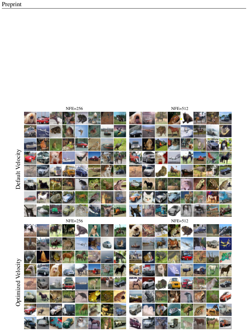
- Metric-induced paths improve quality at low numbers of sampling steps and beat the masked baseline on CIFAR-10 and face-blurred ImageNet-256.
- Permutation-invariant discrete flow matching with kinetic-optimal schedulers reaches state-of-the-art stability rates in inorganic crystal generation.
Reading between the lines
- Editorial inference: the same machinery could be applied to other discrete spaces with natural distances, such as audio tokens or molecular graphs, by plugging a metric into the metric-induced path (27).
- Editorial inference: the proof of optimality depends on the chosen weight $1/p_t(x)$; a data-driven or task-driven weight would likely produce different schedulers while leaving the fixed-path velocity formula intact.
- Editorial inference: the paper's split into a probability-advancing flux and a probability-preserving corrector suggests a general sampling strategy, kinetic-optimal velocity at coarse steps plus symmetric corrector flux at fine steps, which could be tested independently on other discrete generators.
Signed reviews
Editorial analysis
A structured set of objections, weighed in public.
Referee Report
Summary. The paper introduces a framework for discrete flow matching with arbitrary probability paths. It derives a closed-form kinetic-optimal velocity for any prescribed path (Eq. 26) and shows that optimizing the same objective over paths yields mixture paths with a source-dependent scheduler (Eq. 33). It also derives a tractable ELBO for mixture paths. Experiments on text, materials, and images show that the proposed paths and velocities often outperform the standard masking construction.
Significance. If the theoretical claims are fully established, the paper makes a significant contribution: it substantially enlarges the design space of discrete diffusion and flow models, provides a principled kinetic-energy criterion for selecting velocities and paths, and demonstrates practical gains across multiple modalities. The convex derivations for strictly positive paths are clean, the closed-form flux in Eq. (26) is elegant, and the tractable ELBO for mixture paths is a useful algorithmic contribution. The empirical validation is broad, spanning text, materials, and images, with several reproducible comparisons against strong baselines.
major comments (3)
- [Section 4.1, Eq. (19)/(26); Appendix B, Prop. B.1] The statement that Eq. (26) is the kinetic-optimal flux for any prescribed probability path is proved only for strictly positive pt. The proof of Proposition B.1 explicitly assumes pt > 0 and uses the strict positivity of rho_t(x,z) = pt(z)/w_t(x,z). For paths with zero-probability states, the objective (19) with w_t(x,z)=1/p_t(x) assigns an infinite coefficient 1/(p_t(x)p_t(z)) to the flux j_t(x,z); if a generating flux must carry mass into a state with p_t(x)=0, as in the masked mixture path at t=0, the objective value is infinite and the optimization problem has no finite-energy solution. The 'safe flux' and limiting arguments given in the text do not establish that Eq. (26) is the minimizer of (19) in this regime. Since the kinetic-optimality label is used to justify the path and scheduler choices, the paper should either prove the zero-probability case by a rigorous approximation argument that preserves a well-defined sense of optimality, or explicitly restrict the optimality theorem to pt>0 and present the general case as a limiting construction.
- [Section 4.2, Eq. (33); Appendix B, Prop. B.2] The same positivity restriction affects the kinetic-optimal path derivation. Proposition B.2 assumes pt>0, and the energy equivalence used in its proof involves terms such as (d/dt sqrt(pt))^2 and intermediate expressions that become 0/0 at times when a state has zero probability, for example at t=0 for a mask source with p(x1)=0. Thus, the claim that mixture paths with the scheduler (33) are kinetic-optimal for the common mask-source case is unsupported by the proof as written. This claim is the main theoretical motivation for preferring these schedulers over masking, so the paper should clarify the exact status of (33) when p(x1)=0 and provide a rigorous justification, or explicitly weaken the claim to a heuristic or a limiting case.
- [Appendix C.3, Eq. (77)] The power-infinity velocity is defined by taking the limit alpha->infinity in Eq. (74), which yields the factor delta_{argmax_s p_t(s)}(x). This is not well-defined when the maximum of p_t is attained by more than one state, which occurs, for instance, for a uniform source at t=0. Without a tie-breaking rule, Eq. (77) is ambiguous, and the experiments in Figures 5-7 that use this velocity are not fully reproducible. The paper should specify how ties are broken or restrict the claim to paths with a unique maximizer.
minor comments (7)
- [Section 4.1] The notation "∂tpt(x)" in Eq. (26) is introduced without definition; please write "∂_t p_t(x)" and state that it denotes the time derivative.
- [Appendix C.3] The sentence "Indeed the above flux satisfy the Continuity Equation and the Rate Conditions as in Indeed the above flux satisfy the Continuity Equation and the Rate Conditions as in equation 17" is duplicated and contains a subject-verb agreement error; it should be corrected.
- [Section 8.1] The sentence "we used linear and kinetic optimal schedulers with mask, p(x) = δm (x), and β0 ∈ {...} source distributions" is confusing because of the comma after "mask"; please rephrase, for example "with a mask source p(x)=δm(x) as well as β0 ∈ {...}".
- [Appendix E.1] The sentence "Our model are on trained OpenWebText" is ungrammatical; it should read "Our models are trained on OpenWebText and FineWeb-Edu."
- [Appendix E.1] The text "we sample t in [0, 1 − 1e−3]" would be clearer with standard notation, e.g., "we sample t in [0, 1−10^{-3}]"; the same applies to similar expressions in the appendix.
- [Figure 2] The middle-panel labels "u_t (p = 1)" and "u_t (p = ∞)" are not explained in the caption; please define p or rename them to match the notation of Eqs. (74)-(77).
- [Section 8.4 and Table 3] The metric-path model was trained for 600 epochs, while the masked and autoregressive baselines were trained for 300 epochs; this training budget discrepancy should be acknowledged in the comparison, as it may affect the reported FID differences.
Circularity Check
No significant circularity: the kinetic-optimal velocity and scheduler derivations are self-contained from the stated objective, with empirical results used only as external validation.
full rationale
The claimed derivation chain is self-contained and does not reduce to its own inputs. Sections 4.1 and 4.2 start from the explicitly stated symmetric kinetic-energy optimization problem (Eq. 19) with weight w_t(x,z) = 1/p_t(x) (Eq. 25), solve the convex problem via the KKT conditions in Propositions B.1 and B.2, and obtain the closed-form flux (Eq. 26) and the kinetic-optimal scheduler (Eq. 33). These quantities are computed from the objective and boundary conditions, not fit to empirical data, so the 'kinetic-optimal' label is a theorem relative to the stated objective rather than a renamed prediction. The weight choice is an assumption that shapes the notion of optimality, but it is an input objective, not a circular reuse of the target result. Recoveries of velocities from Campbell et al. (2024) and Gat et al. (2024) are consistency checks, not load-bearing self-citations. The ELBO (Eq. 37) is derived in Appendix D from the CTMC variational bound and independently recovers Shi et al. (2024) in the masked special case; its use in training and evaluation is standard rather than circular. Empirical comparisons against SEDD, MD4, LlamaGen, and other external baselines provide independent validation. The zero-probability extension of Proposition B.1 is a proof-technicality concern about safe-flux limiting, not a circularity, because it concerns the rigor of the optimality claim rather than the derivation depending on its conclusion.
Assumptions & free parameters
free parameters (5)
- Text source distribution inverse temperature beta0 =
Selected from {-0.5, 0, 0.5, 1, 2, 4, 64, 256, 1024}; best results around 1024
- CIFAR metric path hyperparameters (lp, a, c) =
lp=3, a=5, c=1
- ImageNet latent metric path hyperparameters (lp, a, c) =
lp=4, a=0.9, c=3
- Velocity family choice alpha=infinity and probability-preserving velocity weight =
Power-infinity flux (Eq. 77) and symmetric corrector (Eq. 35) with varying weights
- Softmax sampling temperature for materials =
0.7 for DFM and KO-DFM, 1.0 for AR
assumptions (6)
- standard math Continuous-time Markov chain generative process with rate conditions (Eqs. 4-5) is a valid model of discrete generative dynamics.
- domain assumption Probability paths factorize across dimensions and velocities change one variable at a time (Eqs. 1, 6, 7).
- ad hoc to paper The symmetric kinetic energy (Eq. 19) with weight w_t(x,z)=1/p_t(x) is the right optimality criterion for selecting velocities and paths.
- standard math The kinetic-optimal relaxation (Prop. B.1) requires p_t>0 and symmetric weights; the extension to zero-probability states uses a safe-flux limiting argument.
- domain assumption User-specified source distributions p(x) and metrics d(x,x1) can be chosen to define useful probability paths.
- standard math The Euler-discretized variational process converges to the CTMC, so the derived ELBO (Eqs. 36-37) is a valid bound.
Cite this review
Pith. "Pith review of Flow Matching with General Discrete Paths: A Kinetic-Optimal Perspective." pith.science (2026). https://pith.science/paper/DVU6JAHP
@misc{pith2026241203487,
  author       = {Pith},
  title        = {Pith review of: Flow Matching with General Discrete Paths: A Kinetic-Optimal Perspective},
  year         = {2026},
  howpublished = {\url{https://pith.science/paper/DVU6JAHP}},
  note         = {Machine review of arXiv:2412.03487}
}
read the original abstract
The design space of discrete-space diffusion or flow generative models are significantly less well-understood than their continuous-space counterparts, with many works focusing only on a simple masked construction. In this work, we aim to take a holistic approach to the construction of discrete generative models based on continuous-time Markov chains, and for the first time, allow the use of arbitrary discrete probability paths, or colloquially, corruption processes. Through the lens of optimizing the symmetric kinetic energy, we propose velocity formulas that can be applied to any given probability path, completely decoupling the probability and velocity, and giving the user the freedom to specify any desirable probability path based on expert knowledge specific to the data domain. Furthermore, we find that a special construction of mixture probability paths optimizes the symmetric kinetic energy for the discrete case. We empirically validate the usefulness of this new design space across multiple modalities: text generation, inorganic material generation, and image generation. We find that we can outperform the mask construction even in text with kinetic-optimal mixture paths, while we can make use of domain-specific constructions of the probability path over the visual domain.
Figures


Figures from the paper (5 more)




Forward citations
Cited by 4 Pith papers
-
UDM-GRPO: Stable and Efficient Group Relative Policy Optimization for Uniform Discrete Diffusion Models
UDM-GRPO is the first RL integration for uniform discrete diffusion models, using final clean samples as actions and forward-process trajectory reconstruction to raise GenEval accuracy from 69% to 96% and OCR accuracy...
-
Structuring The Future: Diffusion LLM Speculative Decoding via Calibrated Draft Graphs
Spiffy speeds up diffusion LLM inference up to about 3x (and up to 7.9x with parallel decoding) by verifying multiple candidate unmasked states in one batched model call, while preserving greedy output.
-
Any-Order Flexible Length Masked Diffusion
FlexMDM is a discrete diffusion model that provably supports any-order generation over variable-length sequences by learning an insertion expectation alongside the unmasking posterior, validated by length-fidelity, ma...
-
Corrector Sampling in Language Models
A training and sampling method that lets autoregressive LLMs resample earlier tokens in a small window, improving reasoning and coding benchmark scores by about 10% relative after a 100B-token fine-tuning.
Reference graph
Works this paper leans on
-
[1]
(1 − δX i t (·)), where λ(X i t |X i
-
[2]
Sample X i t+h ∼ e−hλ(X i t |X i 1)δX i t (·) + (1 − e−hλ(X i t |X i 1)) ut(·,X i t |X i 1) λ(X i t |X i
-
[3]
Coverage Precision & Recall: Precision and Recall metrics computed by comparing 10000 generated structures to the MP-20 test set. Precision is the percentage of generated struc- tures that are close to some test structure, while recall is the percentage of test structures 23 Preprint which are close to some generated structure. Closeness is evaluated usin...
work page 2020
-
[4]
Interpreting this expression, e−hλ(X i t |X i
= ut(X i t , Xi t |X i 1) . Interpreting this expression, e−hλ(X i t |X i
-
[5]
If we do not change state, then we sample from δX i t (·)
is the probability the state does not change. If we do not change state, then we sample from δX i t (·). If we do change state, then we sample from ut(·,X i t |X i 1) λ(X i t |X i
-
[6]
This is still a first-order sampling scheme, i.e
(1 − δX i t (·)), which is a normalized distribution over all states not equal to X i t. This is still a first-order sampling scheme, i.e. it is o(h) error from P(X i t+h | X i t ). However, unlike the simple Euler procedure, this alternative is always a valid PMF for any step size h. Algorithm 1 Euler Solver Require: model θ, x0, h t ← 0 Xt ← x0 while t ...
work page 2024
-
[7]
(δxi 1 (xi) − δzi (xi))pi 1|t(xi 1|z) = ˙κt(xi) 1 − κt(xi) pi 1|t(xi|z) − δzi (xi) X xi 1∈T ˙κt(xi 1) 1 − κt(xi
-
[8]
pi 1|t(xi 1|z). (73) C.3 P OWER ∞ VELOCITY FOR GENERAL PATHS We begin by defining a single parameter family of kinetic optimal velocities. For every α >1 the flux as in equation 22 for τt(x) = pα t (x) is j⋆ t (x, z) = pα t (x)pα t (z) [ft(x) − ft(z)]+ , f t(x) = 1P s∈T pα t (s) ˙pt(x) pα t (x) . (74) Further simplifying j⋆ t (x, z), j⋆ t (x, z) = ˙pt(x) ...
Show all 47 references
-
[9]
Also let qk+1|k(xi|zi, xi
(78) 19 Preprint D E VIDENCE LOWER BOUND (ELBO) FOR CTMC Let 0 = t0 < t1 < · · ·< tK = 1 be a uniform discretization of the interval [0, 1] with h = tk+1 − tk = 1 K . Also let qk+1|k(xi|zi, xi
-
[10]
= δzi (xi) +hut(xi, zi|xi
-
[11]
be the Euler discretization of the variational process, and let pk+1|k(xi|zi) = δzi (xi) + hui t(xi, z) be the Euler discretization of the learned process, with both starting at the same source distribution q0(xi|xi
-
[12]
We also assume the model p(xi 1|xi 0:K) = δxi K (xi 1)
= p(xi). We also assume the model p(xi 1|xi 0:K) = δxi K (xi 1). The discrete-time ELBO is then log pθ(x1) ≥ Ex0:K ∼q0:K (·|x1) [log p(x1|x0:K) + logp0:K(x0:K) − log q0:K(x0:K|x1)] (79) = Ex1:K ∼q1:K (·|x1) DX i=1 " log δxi K (xi
-
[13]
− K−1X k=0 DKL(qk+1|k(xi k+1|xk, xi 1)∥pk+1|k(xi k+1|xk)) # (80) − DX i=1 DKL(q0(xi|xi 1)∥p(xi)) (81) Each term in the summation: DKL(qk+1|k(xi|z, xi 1)∥pk+1|k(xi|z)) (82) = X xi qk+1|k(xi|z, xi
-
[14]
log qk+1|k(xi|z, xi 1) pk+1|k(xi|z) (83) = X xi δzi (xi) + hui t(xi, zi|xi 1) log δzi (xi) + hui t(xi, zi|x1) δzi (xi) + hui t(xi, z) (84) = 1 + hut(zi, zi|xi 1) log 1 + hui t(zi, z|xi 1) 1 + hui t(zi, z) + h X xi̸=zi ut(xi, zi|xi 1) log ui t(xi, zi|xi 1) ui t(xi, z) (85) Tayl...
-
[15]
− hui t(zi, z)) + h X xi̸=zi ui t(xi, zi|xi 1) log ui t(xi, zi|xi 1) ui t(xi, z) + o(h) (88) = h ui t(zi, zi|xi
-
[16]
− ui t(zi, z) + X xi̸=zi ui t(xi, zi|xi 1) log ui t(xi, zi|xi 1) ui t(xi, z) + o(h) (89) Taking limit as K → ∞, hence h = 1 K → 0, and asserting that q(xi K|xi
-
[17]
= δxi 1 (xi K) in this continuous-time limit, we obtain the ELBO: log pθ(x1) ≥ (90) Z 1 0 Ext∼pt(·|x1) DX i=1 ui t(xi t, xt) − ui t(xi t, xi t|xi
-
[18]
+ X x̸=xt ui t(xi, xi t|xi
-
[19]
Assuming the model is such that pθ 1|t(zi|x) = δxi 1 (zi) if xi is unmasked (i.e
log ui t(xi, xt) ut(xi, xi t|xi 1) dt (91) D.1 ELBO FOR MASKED MODELS The masked probability path is as in equation 2 with source distributionpi(xi) = δm (xi). Assuming the model is such that pθ 1|t(zi|x) = δxi 1 (zi) if xi is unmasked (i.e. xi = xi 1), our ELBO as in 20 P...
2024
-
[20]
However for every token independent scheduler κt(xi
will results in a different conditional probability path and hence a different different ELBO. However for every token independent scheduler κt(xi
-
[21]
For token dependent schedulers we only use the Kinetic Optimal scheduler as in equation 33, κt(xi
≡ κt we can change the integration variable from t to κ, log pθ 1(x1) ≥ Z 1 0 dtExt∼pt(·|x1) NX i=1 ˙κt(xi t) 1 − κt(xi t) pθ 1|t(xi t|xt) − X yi ˙κt(yi) 1 − κt(yi) pθ 1|t(yi|xt)+ (94) + (1 − δxi 1 (xi t)) ˙κt(xi 1) 1−κt(xi 1) 1 + logpθ 1|t(xi 1|xt) (95) = Z 1 0 dtExt∼pt(·|x1)...
-
[22]
= sin2(1 − t)Ω(xi 1) sin2 Ω(xi
-
[23]
{i/10:.1f}
= arccos q p(xi 1). (100) 21 Preprint Note that Ω ∈ 0, π 2 , depending on p p(xi 1), we take Ω = π 4 and evaluate the integral, log pθ 1(x1) ≥ Z 1 0 dtExt∼pt(·|x1) NX i=1 ˙κt(xi t) 1 − κt(xi t) pθ 1|t(xi t|xt) − X yi ˙κt(yi) 1 − κt(yi) pθ 1|t(yi|xt)+ (101) + (1 − δxi 1 (xi t))...
2024
-
[24]
Structural Validity: Percentage of generated materials where all pairwise interatomic dis- tances are greather than 0.5 ˚A
-
[25]
Compositional Validity: Percentage of generated materials that are determined to be charge- neutral using the SMACT heuristic system Davies et al. (2019)
2019
-
[27]
Wasserstein Distances of Property Distributions : Wasserstein distances between the dis- tribution of computed properties between the test set and the generated materials. We compute these distances for two properties: density (ρ), and number of unique atoms (Nel) We emphasize...
2021
-
[28]
(2024): (i) We replace the first layer with an embedding table of size 256 × 96, and we stack the channel features such that the input to the U-Net is of shape 288 × 32 × 32
Additionally, we make two changes to the architecture as done in Gat et al. (2024): (i) We replace the first layer with an embedding table of size 256 × 96, and we stack the channel features such that the input to the U-Net is of shape 288 × 32 × 32. (ii) We enlarge the size o...
2024
-
[30]
Generality of probability paths.SEDD starting point is a diffusion matrixQi t(xi, zi) and re- quires a closed-form conditional probability pt(xi|xi
-
[31]
This entails solving a (general) |T |dimensional ODE which can be hard to do in closed form
path solving the Kolmogorov equa- tion (linear ODE) with this rate matrix. This entails solving a (general) |T |dimensional ODE which can be hard to do in closed form. Therefore SEDD resorts to rates of the form Qi t(xi, zi) = σtQi(xi, zi). In contrast, our method offers a clo...
-
[32]
The concrete score function is a particular way to parameterize a probability velocity which is given by ui t(xi, z) = Qi t(xi, zi)si t(xi, z)
Score-velocity conversion. The concrete score function is a particular way to parameterize a probability velocity which is given by ui t(xi, z) = Qi t(xi, zi)si t(xi, z). (109)
-
[33]
The training loss of SEDD can be seen as instance of our ELBO (36) when using the concrete score parameterization
Loss. The training loss of SEDD can be seen as instance of our ELBO (36) when using the concrete score parameterization. Probability velocity vs. concrete score. Using our notation, the noising process of SEDD taking a distribution p1 at time t = 1 , to a some simple distribut...
-
[34]
= Qt(zi, xi) pt(xi|xi 1) pt(zi|xi
-
[35]
The conditional probability path
(120) Considering equation 9, we see that the relation between the concrete score and the probability velocity in equation 118 holds only if Qi t(xi, zi) is independent of x1. The conditional probability path. The conditional probability path is the marginal of the nois- ing p...
-
[36]
(123) The ODE in equation 123 is still too hard to solve in the general case, and some extra assumptions are in order if we hope to solve this equation in analytically
= X zi∈T Qi 1−t(xi, zi)p1−t(zi|xi 1). (123) The ODE in equation 123 is still too hard to solve in the general case, and some extra assumptions are in order if we hope to solve this equation in analytically. SEDD suggests the standard extra assumption that Qi t(xi, zi) = σtQi(x...
-
[37]
(125) The assumption in (124) significantly restricts the space of conditional probability paths
= exp Z t 0 σsds Qi (xi, xi 1). (125) The assumption in (124) significantly restricts the space of conditional probability paths. In contrast, our point of view is arguably simpler: We start with an arbitrary conditional pt(xi|xi 1) and develop a closed-form expression for its...
-
[38]
− d(xi, xi 1)]+, (126) assuming the diffusion matrix Qt(xi, zi) is restricted to Equation (124) we have that Qi(zi, xi) = pt(zi|xi 1) σt ˙βt[d(zi, xi
-
[39]
27 Preprint SEDD training loss
− d(xi, xi 1)]+ (127) on leading to a contradiction since the L.H.S is constant in time. 27 Preprint SEDD training loss. We derive the ELBO train loss for concrete score function as suggested in Lou et al. (2024) from our ELBO (36). To instantiate our ELBO we need to consider ...
2024
-
[40]
= σtQi(zi, xi) pt(xi|xi 1) pt(zi|xi
-
[41]
(129) Now we substitute the velocities in the ELBO (36), log p1(x1) ≥ Z 1 0 Ext∼pt(·|x1) DX i=1 X yi̸=xi t ui t(yi, xi t|xi
(128) The second correspond to the noising process (110) with the boundary condition p1 ≡ q (i.e., data distribution), ui t(xi, z) = σtQi(zi, xi)si t(xi, z). (129) Now we substitute the velocities in the ELBO (36), log p1(x1) ≥ Z 1 0 Ext∼pt(·|x1) DX i=1 X yi̸=xi t ui t(yi, xi t|xi
-
[42]
− ui t(yi, xt) (130) + ui t(yi, xi t|xi
-
[43]
log ui t(yi, xt) ui t(yi, xi t|xi 1) dt (131) = Z 1 0 Ext∼pt(·|x1) DX i=1 X yi̸=xi t σtQi(xi t, yi) pt(yi|xi 1) pt(xi t|xi
-
[44]
− si t(yi|xt) (132) + pt(yi|xi 1) pt(xi t|xi
-
[45]
log pt(xi t|xi 1) pt(yi|xi
-
[46]
si t(yi|xt) dt (133) = Z 1 0 Ext∼pt(·|x1) DX i=1 X yi̸=xi t σtQi(xi t, yi) − si t(yi|xt) (134) + pt(yi|xi 1) pt(xi t|xi
-
[47]
28 Preprint G A DDITIONAL TABLES AND FIGURES NFE=64 NFE=128 Default Velocity NFE=64 NFE=128 Optimized Velocity Figure 5: CIFAR10 Samples for 64 and 128 NFE, default velocities vs
log si t(yi|xt) − g pt(yi|xi 1) pt(xi t|xi 1) dt, (135) where g(s) = s(log(s) − 1). 28 Preprint G A DDITIONAL TABLES AND FIGURES NFE=64 NFE=128 Default Velocity NFE=64 NFE=128 Optimized Velocity Figure 5: CIFAR10 Samples for 64 and 128 NFE, default velocities vs. optimized vel...
2024
-
[2014]
Patryk Chrabaszcz, Ilya Loshchilov, and Frank Hutter
URL https://arxiv.org/abs/1312.3005. Patryk Chrabaszcz, Ilya Loshchilov, and Frank Hutter. A downsampled variant of imagenet as an alternative to the cifar datasets. arXiv preprint arXiv:1707.08819, 2017. Xiaoliang Dai, Ji Hou, Chih-Yao Ma, Sam Tsai, Jialiang Wang, Rui Wang, P...
2017 arXiv
-
[2024]
Following the guidance of (Sun et al., 2024), the autoregressive and masked models were trained for 300 epochs
used. Following the guidance of (Sun et al., 2024), the autoregressive and masked models were trained for 300 epochs. We found that the metric path model benefited from further training, so we trained this variant for 600 epochs. The DFM models required minor architecture adju...
2024
Reviewed August 11, 2026 · model on record in the stance chip above.
Discussion (0). Continue with ORCID to comment.