REVIEW 4 major objections 5 minor 88 references
Backpropagating through a PDE solver during PGD attacks yields stronger, steadier attack losses for neural operators, and training on the resulting hardest samples improves out-of-distribution generalization.
Reviewed by Pith at T0; open to challenge. T0 means a machine referee read the full paper against a public rubric. the ladder, T0–T4 →
T0 review · deepseek-v4-flash
2026-08-04 08:44 UTC pith:EJJZISTC
load-bearing objection The with-solver attack comparison is a real step beyond the dictionary-based baseline for neural operators, but the abstract promises more than the experiments deliver and the solver-gradient path itself is never validated. the 4 major comments →
Solver-Integrated Adversarial Attacking and Training of Neural Operators
The pith
A machine-rendered reading of the paper's core claim, the machinery that carries it, and where it could break.
Core claim
The central claim is that adversarial robustness and generalization of neural operators should be evaluated against the true solver, not a fixed or surrogate ground truth. Defining the loss as the squared model-solver error, ℓ(a)=‖G(a)−g(a)‖², the gradient involves the difference of Jacobians, 2(J_G(a)−J_g(a))ᵀ(G(a)−g(a)). Omitting the solver Jacobian (detached) or replacing the solver with a nearest-neighbor dictionary proxy can underestimate or mislead attacks, especially in 2D Navier–Stokes, where later solver frames carry most of the information. The paper claims that the solver-integrated attack finds larger final losses and more informative perturbed inputs, and that adversarial traini
What carries the argument
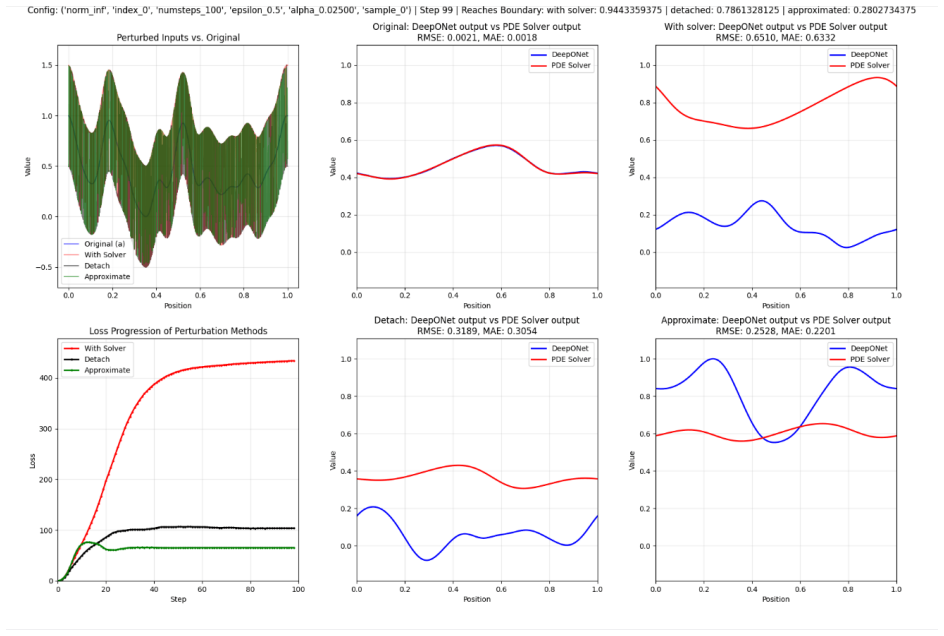
The carrying object is the model-solver error operator with its Fréchet derivative: ℓ(a)=‖G(a)−g(a)‖², whose gradient is 2(J_G−J_g)ᵀ(G−g). Three gradient modes are compared: full backpropagation through both the operator and the solver ('with solver'), detachment of the solver, and a dictionary proxy for the solver. The attack is projected gradient descent in an L2 ball with Adam-style updates, a 10-step cap, and adaptive time-stepping to handle solver blow-up. For the 2D periodic Navier–Stokes case, a soft-DTW loss—a differentiable alignment loss—is used so that pure spatial translations of the solution are not counted as large errors. The neural operators studied are Fourier Neural Operato
Load-bearing premise
Backpropagating through thousands of solver time steps yields gradients that reliably locate worst-case inputs, and the solver's output for those perturbed inputs is accurate enough to serve as ground truth; if long-horizon solver gradients are unstable or uninformative, the claimed advantage of the with-solver attack and the value of its selected samples collapse.
What would settle it
Compute finite-difference directional derivatives of the solver loss at several PGD iterates; if the backpropagated gradient's sign or magnitude disagrees with the finite-difference estimate on a nontrivial fraction of inputs, the with-solver attack is not actually finding worst-case inputs. Alternatively, on a PDE with a computable or enumerable worst-case perturbation, check whether the with-solver attack attains higher true loss than detached or random perturbations of the same norm.
If this is right
- Robustness evaluations that freeze the solver's ground truth can overstate a neural operator's robustness, because the true solver output shifts with the input.
- Solver-selected adversarial samples can act as automatic active-learning data: retraining on them, round by round, reduces out-of-distribution errors for most tested ranges and kernels relative to vanilla training.
- The formulation extends to any regression setting with a differentiable ground-truth oracle, so the method is not tied to PDEs.
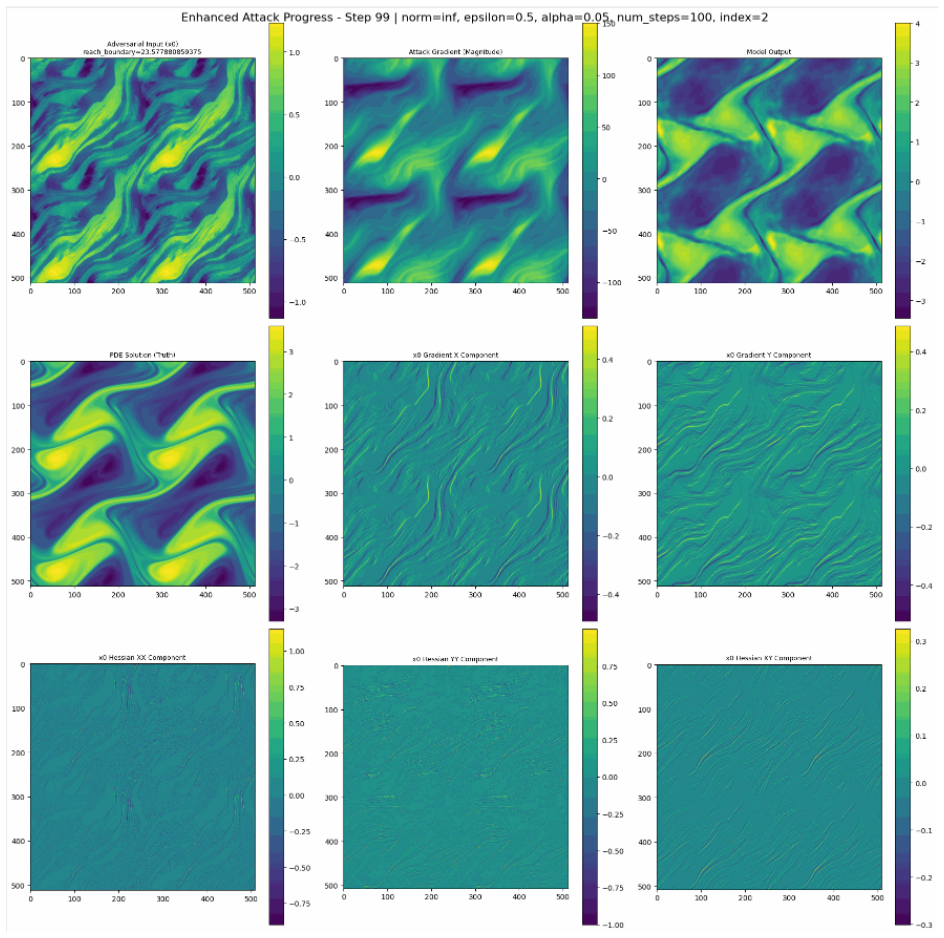
- Averaged adversarial perturbations in the Navier–Stokes experiments reflect the external forcing of the system, and become random fields without forcing, suggesting the attack tracks physically meaningful sensitivity.
- Batch-by-batch adversarial training and random-constant augmentation can worsen in-distribution train/test loss, so the training strategy—not just the attack—determines whether the method helps.
Where Pith is reading between the lines
- The with-solver attack could serve as a probe for which input-space directions a surrogate model gets wrong; the forcing-alignment observation suggests these directions correspond to physically meaningful sensitivities rather than arbitrary noise.
- The large cost of backpropagating through all solver time steps motivates checkpointed, implicit, or adjoint differentiation of the solver; if long-horizon gradients are unstable, hybrid attacks combining finite-difference and backpropagated information may be needed.
- In near-linear regimes, detached and with-solver gradients may nearly coincide, so the practical advantage of full solver backpropagation is most likely to appear in strongly nonlinear, sensitive dynamics—this could be tested as a cheaper diagnostic.
- Random-constant augmentation helped range-shifted inputs but not kernel-shifted ones; combining random augmentation with solver-selected adversarial samples might yield a training distribution with both broad support and hard-case focus.
Editorial analysis
A structured set of objections, weighed in public.
Referee Report
Summary. The manuscript (full-text title "Towards Universal Solvers: Using PGD Attack in Active Learning to Increase Generalizability of Neural Operators as Knowledge Distillation from Numerical PDE Solvers") proposes a PGD-style attack in which the attack loss is computed against a differentiable PDE solver (Exponax) and gradients are backpropagated through both the neural operator and all solver time steps. It compares this "with-solver" attack with a detached-solver variant and a dictionary-approximated variant on 1D Burgers and 2D Navier-Stokes, reporting that the with-solver attack gives faster and larger loss increases. It then presents two retraining schemes (round-by-round active learning and batch-by-batch adversarial training) plus a random-constant augmentation baseline, and reports that round-by-round retraining, especially at round 6, reduces OOD test error on many but not all shifted datasets, while the other two schemes hurt in-distribution performance. The paper also includes extensive appendices on spectral GRF generation and pseudo-spectral solvers.
Significance. If the central empirical claim is correct, the differentiable-solver PGD attack offers a concrete way to mine worst-case samples for neural operators and to use them in active learning, potentially improving OOD robustness. The paper should be credited for: (i) clearly distinguishing with-solver, detached, and dictionary-approximated attack gradients; (ii) reporting timing/memory breakdowns (Tables 1-3); (iii) documenting a falsifiable observation that adversarial perturbations reflect the Navier-Stokes external forcing; and (iv) making explicit that relative FNO loss can mask larger absolute errors. These are useful contributions. However, the manuscript currently resembles an extended technical report: the formalization advertised in the abstract is absent, the training evaluation is statistically thin, and the key gradient-fidelity assumption is unchecked. The contribution is promising but not yet established.
major comments (4)
- [Title/Abstract vs. Methods] The arXiv abstract claims the paper "formalizes the definition of generalization and robustness through a model-solver error operator" and identifies norm-bounded attack-loss increase and Jacobian-error function norm as robustness metrics. The full text contains no such formalization: no model-solver error operator is defined, and no theorem or definition links the proposed MSE loss to the claimed generalization/robustness metrics. The Methods section defines Fréchet derivatives and batch derivatives (the equations for ℓ(a)) but never uses them to state the advertised formal definitions. Since the abstract's formalization is a central advertised contribution, this unbacked claim must either be removed or actually provided in a revision.
- [Adversarial Training Using Above PGD Attack] The central training claim is not supported by the reported numbers. The text says batch-by-batch and random-constant training "cause greater loss in the original train and test datasets," and that round-by-round achieves lower loss for "nearly all datasets except range (-1.5,-1)" only at the 6th round; it also says results "increase the loss of many datasets while decrease the loss of others." Figure 5 is a single loss-change plot with no numerical values, no error bars, no multiple seeds, and no statistical tests. Moreover, batch-by-batch training is forced to batch size 2 while the original FNO training uses batch size 20, confounding the comparison. The conclusion that solver-integrated adversarial training "clearly improves both generalizability and robustness" is therefore overstated and requires quantitative tables and repeated-run statistics.
- [Challenges in the Above PGD Attack] The with-solver attack's advantage rests on gradients backpropagated through all ~4000 solver time steps (Tables 1-3). The paper does not validate the fidelity of these gradients. It concedes the need for adaptive time-step shrinking, a 10-step limit, and fallback to the last non-blow-up input. Without a check against a non-gradient search (e.g., random or coordinate ascent within the same ε-ball) or a finite-difference verification on a reduced problem, the larger attack losses in Figures 17-36 and the samples selected for round-by-round training may reflect numerical artifacts of the unrolled solver Jacobian rather than true worst-case model-solver discrepancy. This is load-bearing for the with-solver advantage and for active-sample selection.
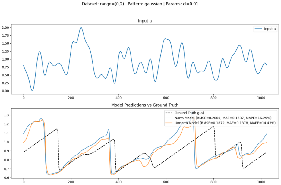
- [Experiments and Evaluation] The empirical evaluation is too thin to support the strong claims. OOD results are reported as plots (Figures 1-2) without dataset sizes, confidence intervals, or repeated training; the qualitative claim that value range dominates is not quantified or compared against kernel-type effects. No code or data release is mentioned, and the model/training hyperparameters for FNO, DeepONet, and Exponax are not specified. The paper's own text notes that attacks on NS require 30-50 GB memory and only batch size 7 fits, yet the effect of these constraints on results is not discussed. In addition, the OOD evaluation uses the same model-solver RMSE/MSE that the training objective optimizes; alternative metrics (e.g., spectral errors or physics-based invariants) are not reported, so it is unclear how much of the improvement is specific to the chosen metric.
minor comments (5)
- [Title/Abstract] The arXiv abstract (with the "Solver-Integrated..." title) and the full-text title/abstract differ substantially. Please reconcile the two and ensure the abstract claims match the content.
- [References] The reference list contains duplicates and incomplete entries: [39] and [40] are the same paper; [9]/[10] are both Soft-DTW; [47]/[48] are both Madry et al.; several entries are incomplete (e.g., "Kong" et al., "et al." placeholders).
- [Algorithm 1] The note "Normalizing d(step 4)" in Algorithm 1 is incorrect; normalization occurs in step 14. The L2 PGD pseudocode and Algorithm 1 also duplicate but differ in Adam details; unify them.
- [Notation and typos] There are numerous typos and inconsistent notations, e.g., "Orzsag" (should be Orszag), "V orticity-Streamfucntion F ormulation", "negand" / "All pos", and inconsistent naming of norms ("norm=2" vs. L2). These should be cleaned up.
- [Figures] Many figure captions omit units or full parameter settings (e.g., Figures 17-36), and several figures lack error bars or repeated-run information. The appendix is also very long and contains tutorial material that could be condensed or moved to supplementary material.
Circularity Check
No significant circularity: the solver is an external oracle and the OOD generalization benchmarks are held out from the training objective.
full rationale
The derivation chain is not circular in the sense that matters here. The adversarial objective and all reported losses are computed against solver outputs g(a) produced by Exponax, an external numerical solver; the learned neural operator is trained to match that solver, and no fitted parameter is later renamed as a prediction. The paper defines generalization as fixed-input model-solver loss, but the OOD test sets use different initial-condition distributions (different GRF kernels, correlation lengths, value ranges) that are not inputs to the minimax objective. Thus the round-by-round improvements on those held-out distributions are not forced by construction. The with-solver attack naturally maximizes the exact loss used to evaluate it, so its larger final attack loss is partly an expected property of first-order optimization rather than an independent discovery; however, this is not a fitted-input-called-prediction circularity, and the central OOD generalization claim does not reduce to this. The acknowledged numerical fragility of backpropagating through roughly 4000 solver timesteps ('The gradient has to be back propagated through all 4000 layers', Challenges section) is a real validation limitation for the method's effectiveness, but it is a correctness/robustness risk, not a circular step. There are no load-bearing self-citations and no imported uniqueness theorems from the authors' own prior work.
Axiom & Free-Parameter Ledger
free parameters (5)
- Attack norm-ball radius epsilon (1D L2=10, L∞=0.5; 2D L2=13.1–78.6, L∞=0.5–1) =
varies per experiment
- PGD step size alpha (0.0025–50) and number of PGD steps T (10–200) =
varies per experiment
- Active-learning round count (best at 6th round) =
6
- Soft-DTW smoothing parameter gamma =
0.01
- Dictionary size for approximated baseline (20 to 20000) =
varied
axioms (4)
- domain assumption Exponax pseudo-spectral solver output g(a) is an accurate ground-truth oracle and is differentiable with respect to input a.
- domain assumption Backpropagating through all 4000 solver timesteps yields gradients that reliably identify worst-case perturbations.
- domain assumption Small L2/L∞ perturbations of initial conditions are physically meaningful and sufficient to expose OOD failures.
- ad hoc to paper Out-of-distribution failure of neural operators is primarily controlled by input value range rather than kernel/spectral shape.
read the original abstract
Neural operators are widely used as fast surrogates for numerical PDE solvers, mapping input functions to solution functions. However, their generalizability and robustness are not yet clearly defined in the operator-learning setting, which differs from traditional adversarial robustness definitions. This paper studies the generalizability and robustness of a learned neural operator from a solver-integrated perspective, addressing the challenge that the output of a learned operator and a numerical solver tends to change in tandem under input perturbation. First, we formalize the definition of generalization and robustness through a model-solver error operator, identifying fixed-input model-solver loss as generalization metric, and norm-bounded adversarial attack loss increase and Jacobian-error function norm as robustness metric. Second, we identify the solver-integrated adversarial attack as appropriate for PDE operator learning and show why model-only or fixed-ground-truth attacks can be insufficient when the solver output also changes with the input. Third, we develop solver-integrated adversarial training methods for neural operators. Experiments on representative PDE benchmarks show that this solver-integrated adversarial training clearly improves both generalizability and robustness. Deeper solver integration yields more effective attacks, more informative samples, and more efficient training than less integrated alternatives. These results provide a general framework for robust operator training and automatic sample selection without heavy manual intervention. More broadly, the formulation applies to adversarial regression whenever a ground-truth oracle can evaluate, and ideally differentiate, the true input-output map; PDE operator learning is one such case.
Figures








Reference graph
Works this paper leans on
-
[1]
Wikipedia, 2025
Dirac comb. Wikipedia, 2025. URLhttps://en.wikipedia.org/wiki/Dirac_comb
2025
-
[2]
Wikipedia, 2025
Mat´ ern covariance function. Wikipedia, 2025. URLhttps://en.wikipedia.org/wiki/Mat%C3%A9rn_ covariance_function
2025
-
[3]
Evaluating the adversarial robustness for fourier neural operator
Adedotun Adesoji et al. Evaluating the adversarial robustness for fourier neural operator. SRML Workshop at ICLR 2022, 2022. URLhttps://arxiv.org/abs/2204.04259
Pith/arXiv arXiv 2022
-
[4]
Deepak Akhare, Pan Du, Tengfei Luo, and Jian-Xun Wang. Implicit neural differential model for spatiotemporal dynamics (im-pindiff).arXiv preprint arXiv:2504.02260, 2025
Pith/arXiv arXiv 2025
-
[5]
Nacime Bouziani, David A. Ham, and Ado Farsi. Differentiable programming across the pde and machine learning barrier.arXiv preprint arXiv:2409.06085, 2024
Pith/arXiv arXiv 2024
-
[6]
Keaton J. Burns, Geoffrey M. Vasil, Jeffrey S. Oishi, Daniel Lecoanet, and Benjamin P. Brown. Dedalus: A flexible framework for numerical simulations with spectral methods.Physical Review Research, 2020. doi: 10.1103/PhysRevResearch.2.023068. URLhttps://arxiv.org/abs/1905.10388
Pith/arXiv arXiv 2020
-
[7]
Canuto, M.Y
C. Canuto, M.Y. Hussaini, A. Quarteroni, and T.A. Zang.Spectral Methods in Fluid Dynamics. Springer, 1988
1988
-
[8]
Clercx et al
Herman J.H. Clercx et al. A spectral solver for the navier–stokes equations in cylindrical geometries. Journal of Computational Physics, 1997. AB2 for advection, Crank–Nicolson for diffusion
1997
-
[9]
Soft-DTW: a differentiable loss function for time-series
Marco Cuturi and Mathieu Blondel. Soft-DTW: a differentiable loss function for time-series. InPro- ceedings of the 34th International Conference on Machine Learning (ICML), pages 894–903, Sydney, Australia, 2017. PMLR
2017
-
[10]
Soft-dtw: a differentiable loss function for time-series
Marco Cuturi and Mathieu Blondel. Soft-dtw: a differentiable loss function for time-series. InProceedings of the 34th International Conference on Machine Learning (ICML), 2017
2017
-
[11]
Nima Hosseini Dashtbayaz, Hesam Salehipour, Adrian Butscher, and Nigel Morris. Physics-informed re- duced order modeling of time-dependent pdes via differentiable solvers.arXiv preprint arXiv:2505.14595, 2025
arXiv 2025
-
[12]
C. R. Dietrich and G. N. Newsam. Fast and exact simulation of stationary gaussian processes through circulant embedding.SIAM Journal on Scientific Computing, 1997
1997
-
[13]
The kernel cookbook: Advice on covariance functions, 2014
David Duvenaud. The kernel cookbook: Advice on covariance functions, 2014. URLhttps://www.cs. toronto.edu/~duvenaud/cookbook/
2014
-
[14]
Fourier series representation of periodic signals
Michael Dzhibladze. Fourier series representation of periodic signals. Purdue University lecture notes,
-
[15]
GitHub / open source
Tum-PBS / Philipp Holl et al.ϕflow: A differentiable pde solving framework. GitHub / open source. Integration with PyTorch, TensorFlow, JAX
-
[16]
Advanced gaussian processes (scribed notes, lecture 21)
Konstantin Genin and Yutong Zheng. Advanced gaussian processes (scribed notes, lecture 21). CMU 10-708 Spring 2015, 2015. URLhttps://www.cs.cmu.edu/ ~epxing/Class/10708-15/notes/10708_ scribe_lecture21.pdf
2015
-
[17]
Goodfellow, Jonathon Shlens, and Christian Szegedy
Ian J. Goodfellow, Jonathon Shlens, and Christian Szegedy. Explaining and harnessing adversarial examples.arXiv preprint arXiv:1412.6572, 2015. URLhttps://arxiv.org/abs/1412.6572
Pith/arXiv arXiv 2015
-
[18]
Discrete fourier transform and wavelet transforms (math 357 notes)
Roe Goodman. Discrete fourier transform and wavelet transforms (math 357 notes). Technical re- port, Rutgers University, 2008. URLhttps://sites.math.rutgers.edu/ ~goodman/pub/math_357_ lectures.pdf. Supplementary class notes, revised May 3, 2008. 20
2008
-
[19]
Finite fourier transform, circulant matrices, and the fast fourier transform
Roe Goodman. Finite fourier transform, circulant matrices, and the fast fourier transform. Techni- cal report, Rutgers University, 2015. URLhttps://sites.math.rutgers.edu/ ~yzhuang/rci/math/ fftnotes.pdf. Supplementary notes for Math 642/550
2015
-
[20]
J. Gou et al. Knowledge distillation: A survey.arXiv preprint arXiv:2006.05525, 2020
Pith/arXiv arXiv 2006
-
[21]
Robert M. Gray. Toeplitz and circulant matrices: A review.Foundations and Trends in Communications and Information Theory, 2(3):155–239, 2006
2006
-
[22]
Muhammad Bilal Hafeez and Marek Krawczuk. A review: Applications of the spectral finite element method.Archives of Computational Methods in Engineering, 2023. doi: 10.1007/s11831-023-09911-2. URLhttps://link.springer.com/article/10.1007/s11831-023-09911-2
-
[23]
Spectral kernels (gpss 2021)
Markus Heinonen. Spectral kernels (gpss 2021). Gaussian Process Summer School slides, 2021. URL https://gpss.cc/gpss21/slides/Heinonen2021.pdf
2021
-
[24]
Distilling the knowledge in a neural network
Geoffrey Hinton, Oriol Vinyals, and Jeff Dean. Distilling the knowledge in a neural network. arXiv preprint arXiv:1503.02531, 2015
Pith/arXiv arXiv 2015
-
[25]
Hou and Ruo Li
Thomas Y. Hou and Ruo Li. Computing nearly singular solutions using pseudo-spectral methods. Communications in Computational Physics, 2007
2007
-
[26]
Mingi Ji, Byeongho Heo, and Sungrae Park. Show, attend and distill: Knowledge distillation via attention-based feature matching.arXiv preprint arXiv:2102.02973, 2021
Pith/arXiv arXiv 2021
-
[27]
Unsupervised learning of full-waveform inversion: Connecting cnn and partial differential equation in a loop.Preprint / Conference (ICLR), 2022
Peng Jin, Xitong Zhang, Yinpeng Chen, Sharon Huang, Zicheng Liu, and Youzuo Lin. Unsupervised learning of full-waveform inversion: Connecting cnn and partial differential equation in a loop.Preprint / Conference (ICLR), 2022
2022
-
[28]
, and Youzuo Lin
Peng Jin, Yinan Feng, . . . , and Youzuo Lin. An empirical study of large-scale data-driven full waveform inversion.Scientific Reports, 14, 2024
2024
-
[29]
Perceptual losses for real-time style transfer and super-resolution.European Conference on Computer Vision (ECCV) Workshops, 2016
Justin Johnson, Alexandre Alahi, and Li Fei-Fei. Perceptual losses for real-time style transfer and super-resolution.European Conference on Computer Vision (ECCV) Workshops, 2016
2016
-
[30]
Cambridge University Press, 3rd edition, 2004
Yitzhak Katznelson.An Introduction to Harmonic Analysis. Cambridge University Press, 3rd edition, 2004
2004
-
[31]
Elastic image matching is np-complete.Pattern Recognition Letters, 24(1-3):445–453, 2003
Daniel Keysers and Walter Unger. Elastic image matching is np-complete.Pattern Recognition Letters, 24(1-3):445–453, 2003
2003
-
[32]
Exponax: Fourier spectral etdrk time-steppers in jax
Florian K¨ ohler. Exponax: Fourier spectral etdrk time-steppers in jax. Online, 2024.https://fkoehler. site/exponax/
2024
-
[33]
et al. Kong. Physics informed adversarial training for solving partial differential equations (piat). arXiv:2207.XXXX, 2022. physics-informed adversarial training (representative early work)
2022
-
[34]
Jeong-Hoe Ku, JiHun Oh, YoungYoon Lee, et al. A selective survey on versatile knowledge distillation paradigm for neural network models.arXiv preprint arXiv:2011.14554, 2020
Pith/arXiv arXiv 2011
-
[35]
Laga and W
I. Laga and W. Kleiber. The modified mat´ ern process.Applied Mathematics and Computation, 2017. URLhttps://amath.colorado.edu/faculty/kleiberw/papers/Laga2017.pdf
2017
-
[36]
Direct image matching by dynamic warping
Hansheng Lei and Venu Govindaraju. Direct image matching by dynamic warping. InProceedings of the International Conference on Pattern Recognition (ICPR), 2003
2003
-
[38]
Adversarial training for physics-informed neural networks (at-pinns), 2023
Yao Li, Shengzhu Shi, Zhichang Guo, and Boying Wu. Adversarial training for physics-informed neural networks (at-pinns), 2023. URLhttps://arXiv.org/abs/2310.11789. Preprint arXiv:2310.11789, https://arxiv.org/abs/2310.11789. 21
arXiv 2023
-
[40]
Zongyi Li, Nikola B. Kovachki, Kamyar Azizzadenesheli, Burigede Liu, Andrew Stuart, Kaushik Bhat- tacharya, and Anima Anandkumar. Fourier neural operator for parametric partial differential equations. arXiv:2010.08895, 2020
Pith/arXiv arXiv 2010
-
[41]
Fourier neural operator with learned deformations for pdes on general geometries.Journal of Machine Learning Research, 2023
Zongyi Li, Daniel Zhengyu Huang, Burigede Liu, and Anima Anandkumar. Fourier neural operator with learned deformations for pdes on general geometries.Journal of Machine Learning Research, 2023. Preprint / JMLR version
2023
-
[42]
et al. Liu. Adaptive movement sampling physics-informed residual network. arXiv:2504.03244, 2025. movement-based residual sampling and domain-coverage constraints
Pith/arXiv arXiv 2025
-
[44]
Lu Lu, Pengzhan Jin, and George Em Karniadakis. Deeponet: Learning nonlinear operators for identi- fying differential equations based on the universal approximation theorem of operators.arXiv preprint arXiv:1910.03193, 2019. URLhttps://arxiv.org/abs/1910.03193. Accessed: 2025-09-27
Pith/arXiv arXiv 1910
-
[45]
Karniadakis
Lu Lu, Pengzhan Jin, and George E. Karniadakis. Learning nonlinear operators via deeponet based on the universal approximation theorem of operators, 2021
2021
-
[46]
Lu Lu, Pengzhan Jin, and George Em Karniadakis. Learning nonlinear operators via deeponet based on the universal approximation theorem of operators, 2021. Preprint / arXiv:2104.09481
Pith/arXiv arXiv 2021
-
[47]
Towards deep learning models resistant to adversarial attacks.arXiv preprint arXiv:1706.06083, 2017
Aleksander Madry, Aleksandar Makelov, Ludwig Schmidt, Dimitris Tsipras, and Adrian Vladu. Towards deep learning models resistant to adversarial attacks.arXiv preprint arXiv:1706.06083, 2017. URL https://arxiv.org/abs/1706.06083. Accessed: 2025-09-27
Pith/arXiv arXiv 2017
-
[48]
To- wards deep learning models resistant to adversarial attacks
Aleksander Madry, Aleksandar Makelov, Ludwig Schmidt, Dimitris Tsipras, and Adrian Vladu. To- wards deep learning models resistant to adversarial attacks. InInternational Conference on Learning Representations (ICLR), 2018. URLhttps://openreview.net/pdf?id=rJzIBfZAb
2018
-
[49]
Majda and Andrea L
Andrew J. Majda and Andrea L. Bertozzi.Vorticity and Incompressible Flow. Cambridge University Press, 2002
2002
-
[50]
Fabien Margairaz, Marco G. Giometto, Marc B. Parlange, and Marc Calaf. Comparison of dealiasing schemes in large-eddy simulation of neutrally stratified atmospheric flows.Geoscientific Model Devel- opment, 11:4069–4084, 2018. doi: 10.5194/gmd-11-4069-2018. URLhttps://gmd.copernicus.org/ articles/11/4069/2018/
-
[51]
Circulant matrices
Department of Mathematics / Course 18.06 MIT. Circulant matrices. Technical report, Massachusetts In- stitute of Technology, 2017. URLhttps://web.mit.edu/18.06/www/Spring17/Circulant-Matrices. pdf. Lecture notes, available at MIT OCW (PDF)
2017
-
[52]
Molenaar
D. Molenaar. Forced navier–stokes flows on a bounded 2d domain: Abcn scheme overview. Technical report, 2004
2004
-
[53]
Mohammad Amin Nabian, Ryan J. Gladstone, and Hadi Meidani. Efficient training of physics-informed neural networks via importance sampling.Computer-Aided Civil and Infrastructure Engineering, 36(8): 962–977, 2021. doi: 10.1111/mice.12685
-
[54]
Learning dtw global constraint for time series classification
Vit Niennattrakul and Chotirat Ann Ratanamahatana. Learning dtw global constraint for time series classification. InProceedings of the 2009 International Conference on Data Mining, 2009. 22
2009
-
[55]
Steven A. Orszag. Numerical methods for the simulation of turbulence. InFluid Dynamics, 1972. Introduces the 2/3 dealiasing rule
1972
-
[56]
K. V. Park et al. Al-pinn: Active learning-driven physics-informed neural networks for efficient sample selection. arXiv:2502.03963, 2025
Pith/arXiv arXiv 2025
-
[57]
Maziar Raissi, Paris Perdikaris, and George E. Karniadakis. Physics informed deep learning (part i): Data-driven solutions of nonlinear partial differential equations.arXiv preprint arXiv:1711.10561, 2017
Pith/arXiv arXiv 2017
-
[58]
Maziar Raissi, Paris Perdikaris, and George E. Karniadakis. Physics-informed neural networks: A deep learning framework for solving forward and inverse problems involving nonlinear partial differential equations.Journal of Computational Physics, 378:686–707, 2019. doi: 10.1016/j.jcp.2018.10.045
-
[59]
Carl Edward Rasmussen and Christopher K. I. Williams.Gaussian Processes for Machine Learning. MIT Press, 2006. URLhttps://gaussianprocess.org/gpml/chapters/RW4.pdf
2006
-
[60]
Williams.Gaussian Processes for Machine Learning
Carl Edward Rasmussen and Christopher K.I. Williams.Gaussian Processes for Machine Learning. MIT Press, 2006
2006
-
[61]
Fitnets: Hints for thin deep nets
Adrian Romero, Nicolas Ballas, Samira E Kahou, Cesar Chassang, Carlo Gatta, and Yoshua Bengio. Fitnets: Hints for thin deep nets. InICLR, 2015
2015
-
[62]
Wiley, 1990
Walter Rudin.Fourier Analysis on Groups. Wiley, 1990
1990
-
[63]
Dynamic programming algorithm optimization for spoken word recog- nition.IEEE Transactions on Acoustics, Speech, and Signal Processing, 26(1):43–49, 1978
Hiroaki Sakoe and Seibi Chiba. Dynamic programming algorithm optimization for spoken word recog- nition.IEEE Transactions on Acoustics, Speech, and Signal Processing, 26(1):43–49, 1978
1978
-
[64]
Dynamic time warping algorithm review
Pavel Senin. Dynamic time warping algorithm review. Technical Report, University of Hawai‘i at M¯ anoa,
-
[65]
Discovering the fourier transform: A tutorial on circulant matrices, circular con- volution, and the dft
Smarker. Discovering the fourier transform: A tutorial on circulant matrices, circular con- volution, and the dft. GitHub gist, 2019. URLhttps://gist.github.com/Smarker/ 1e6fb0ebfd43778b535cc049868589f3. Online tutorial note
2019
-
[66]
Understanding gaussian process regression using the fourier transform, 2000
Peter Sollich. Understanding gaussian process regression using the fourier transform, 2000. URLhttps: //homepages.inf.ed.ac.uk/ckiw/postscript/sheff3.pdf. Lecture notes
2000
-
[67]
Fourier-spectral methods for navier–stokes equations in 2d
Mashbat Suzuki. Fourier-spectral methods for navier–stokes equations in 2d. Course notes/technical report, McGill University (MATH 595), 2014. URLhttps://www.math.mcgill.ca/gantumur/ math595f14/NSMashbat.pdf. December 17, 2014
2014
-
[68]
Nils Thuerey, Philipp Holl, Maximilian Mueller, Patrick Schnell, Felix Trost, and Kiwon Um. Physics- based deep learning. arXiv preprint, 2021. URLhttps://arxiv.org/abs/2109.05237
Pith/arXiv arXiv 2021
-
[69]
Trefethen.Spectral Methods in MATLAB
Lloyd N. Trefethen.Spectral Methods in MATLAB. SIAM, 2000
2000
-
[70]
Physics-informed neural network with adaptive mesh refinement sampling
Jakub Trynda. Physics-informed neural network with adaptive mesh refinement sampling. SSRN preprint 5148446, 2024
2024
-
[71]
Solver-in-the- loop: Learning from differentiable physics to interact with iterative pde-solvers
Kiwon Um, Robert Brand, Yun (Raymond) Fei, Philipp Holl, and Nils Thuerey. Solver-in-the- loop: Learning from differentiable physics to interact with iterative pde-solvers. InNeurIPS, 2020. https://proceedings.neurips.cc/paper/2020/file/43e4e6a6f341e00671e123714de019a8-Paper.pdf
2020
-
[72]
Generalized harmonic analysis.Acta Mathematica, 1930
Norbert Wiener. Generalized harmonic analysis.Acta Mathematica, 1930. Wiener–Khinchin link ACF↔PSD
1930
-
[73]
Andrew Gordon Wilson and Ryan P. Adams. Gaussian process kernels for pattern discovery and ex- trapolation, 2013. URLhttps://arxiv.org/abs/1302.4245
Pith/arXiv arXiv 2013
-
[74]
Andrew Gordon Wilson and Ryan P. Adams. Gaussian process kernels for pattern discovery and ex- trapolation. InProceedings of the 30th International Conference on Machine Learning (ICML). PMLR,
-
[75]
Andrew Gordon Wilson and Eric P. Xing. Advanced gaussian processes (lecture slides). CMU 10-708 Spring 2015, 2015. URLhttps://www.cs.cmu.edu/ ~epxing/Class/10708-15/slides/andrewgp2. pdf
2015
-
[76]
Wood and Grace Chan
Andrew T.A. Wood and Grace Chan. Simulation of stationary gaussian vector fields.Statistics and Computing, 1994
1994
-
[78]
Chenxi Wu, Min Zhu, Qinyang Tan, Yadhu Kartha, and Lu Lu. A comprehensive study of non- adaptive and residual-based adaptive sampling for physics-informed neural networks.Computer Meth- ods in Applied Mechanics and Engineering, 403:115671, 2023. doi: 10.1016/j.cma.2022.115671. URL https://arxiv.org/abs/2207.10289. Accessed: 2025-09-27
arXiv 2023
-
[79]
On the generalization properties of adversarial training
Yue Xing, Qifan Song, and Guang Cheng. On the generalization properties of adversarial training. In Proceedings of the 24th International Conference on Artificial Intelligence and Statistics (AISTATS), pages 505–513, 2021. URLhttps://proceedings.mlr.press/v130/xing21b.html
2021
-
[80]
Jeremy Yu, Lu Lu, Xuhui Meng, and George E. Karniadakis. Gradient-enhanced physics-informed neural networks for forward and inverse pde problems.Computer Methods in Applied Mechanics and Engineering, 393:114823, 2022. doi: 10.1016/j.cma.2022.114823
arXiv 2022
-
[81]
Dongkun Zhang, Li Guo, and George E. Karniadakis. Quantifying total uncertainty in physics-informed neural networks for solving forward and inverse stochastic problems.Journal of Computational Physics, 397:108850, 2019. doi: 10.1016/j.jcp.2019.07.048
-
[82]
Adversarial training: A survey.arXiv preprint arXiv:2410.15042, 2024
Mengnan Zhao, Lihe Zhang, Jingwen Ye, Huchuan Lu, Baocai Yin, and Xinchao Wang. Adversarial training: A survey.arXiv preprint arXiv:2410.15042, 2024. URLhttps://arxiv.org/abs/2410.15042
Pith/arXiv arXiv 2024
-
[83]
Improving generalization of adversarial training via robust critical fine-tuning
Kai Zhu et al. Improving generalization of adversarial training via robust critical fine-tuning. InICCV 2023, 2023. URLhttps://openaccess.thecvf.com/content/ICCV2023/papers/Zhu_Improving_ Generalization_of_Adversarial_Training_via_Robust_Critical_Fine-Tuning_ICCV_2023_ paper.pdf. 24 Appendix: Pseudospectral Methods and Spectral GRF Generation A 1D Burgers...
2023
-
[86]
For FFT libraries using real-to-complex transforms (e.g
Build wavenumber arraysk x, ky andk 2. For FFT libraries using real-to-complex transforms (e.g. RFFT), store the half-spectrum indexing accordingly (truncate the redundant half along the last di- mension). Setk 2(0,0)←1 for safe division, and later force bψ(0,0) = 0
discussion (0)
Sign in with ORCID, Apple, or X to comment. Anyone can read and Pith papers without signing in.