Cosmological Parameter Estimation with Sequential Linear Simulation-based Inference

Nicolas Mediato-Diaz; Will Handley

REVIEW 4 major objections 6 minor 31 references

Cosmological Parameter Estimation with Sequential Linear Simulation-based Inference

T0 review · 4 major / 6 minor · reviewed 2026-08-10 · deepseek-v4-flash

Challenge this review Re-run · record.json Download PDF Read on arXiv ↗ Review JSON

Pith's one-line read This paper argues that fast, explainable simulation-based inference can be achieved by replacing neural density estimators with a sequentially updated linear-Gaussian likelihood, reaching nested-sampling-quality CMB posteriors in about…

desk verdict An honest, modest SBI baseline built on standard Bayesian linear regression; the calibration claim in the CMB section is not yet supported. read the letter →

arxiv 2501.03921 v1 pith:ERA6G6KQ submitted 2025-01-07 astro-ph.IM astro-ph.COphysics.data-anstat.ML

Nicolas Mediato-Diaz , Will Handley This is my paper · ORCID

classification astro-ph.IMastro-ph.COphysics.data-anstat.ML

keywords simulation-basedinferencelinearlikelihoodapproximationsequentialBayesianparameterestimationCMBpowerspectrumneuraldensityexplainableCosmo

verification ladder T0 review T1 audit T2 compute T3 formal

The pith

A machine-rendered reading of the paper's core claim, the machinery that carries it, and where it could break.

The reading

The paper introduces Linear Simulation-based Inference (LSBI), a likelihood-free parameter estimation method that approximates the simulator's output as a Gaussian whose mean is linear in the parameters. It derives closed-form posterior distributions for the unknown linear-likelihood hyper-parameters directly from simulator samples, then iterates the procedure around the observed data to handle nonlinear models. On toy models and an emulated CMB temperature power spectrum, four or five rounds of roughly ten thousand simulations per round produce posteriors that agree with nested sampling while remaining fully explainable. The broader point is that fast simulation-based inference does not require a neural network, which addresses the lack of intellectual oversight that black-box approaches can create.

What carries the argument

The load-bearing object is the linear simulation-based likelihood, $D|\theta \sim \mathcal{N}(m + M\theta, C)$, with hyper-parameters $m$, $M$, and $C$ treated as unknown. The paper derives their posterior distributions directly from simulator samples (Eqs. 13\textendash 15), avoiding neural density estimation; the sequential version then uses the previous posterior as the sampling distribution for the next round's simulations, which is what makes the linear approximation hold for nonlinear models. This machinery converts simulation-based inference into a sequence of closed-form Gaussian, matrix-normal, and inverse-Wishart updates.

What would settle it

Run sequential LSBI on a realistic CMB likelihood that includes non-Gaussian foreground and beam systematics and compare to nested sampling after five rounds of $10^4$ simulations; if the KL divergence does not approach the nested-sampling value, the paper's central claim that LSBI is competitive on realistic cosmological data is falsified.

Watch

Extended reading notes

Core claim

Under the linear-Gaussian approximation $D|\theta \sim \mathcal{N}(m + M\theta, C)$, LSBI obtains closed-form posteriors for the unknown likelihood hyper-parameters from $k$ simulated pairs $\{(\theta^{(i)}, D^{(i)})\}$: $m$ is Gaussian, $M$ is matrix-normal, and $C$ is inverse-Wishart (Eqs. 13\textendash 15). The parameter posterior is then a Gaussian mixture obtained by sampling these hyper-parameter posteriors. Sequentially re-running LSBI with simulation parameters drawn from the previous round's posterior narrows the region where the linear approximation is valid, and on the CMB power spectrum this converges after four or five rounds of $10^4$ simulations to posteriors consistent with nested sampling. The paper claims this makes fast, credible simulation-based inference achievable without neural networks and with full explainability.

Load-bearing premise

The method assumes that, within each round, the simulator's output is well described by a Gaussian whose mean is linear in the parameters; if the true noise has undefined variance (as with Cauchy noise) or the model is strongly nonlinear over the sampled region, the approximation breaks down.

Editorial extensions

If this is right

Sequential LSBI reaches the same posterior as nested sampling with a total simulation budget of roughly four to five times $10^4$ calls on the CMB temperature power spectrum, comparable to neural density estimators.
The method tolerates deviations from Gaussian noise: uniform and Student-$t$ noise cases converge after about four rounds, while asymmetric Laplacian noise shows slower but still useful convergence.
Because the posterior is a Gaussian mixture over analytically sampled hyper-parameters, the computation can be parallelized and does not require training a neural network.
The same framework yields an estimate of the Bayesian evidence, so model comparison can in principle be performed without additional simulator calls.
A minimum of $k_{\min} = n + 2d + 2$ simulations is required for well-defined distributions, and the recommended number of hyper-parameter samples $N$ is of order $10^3$ to avoid overconfidence.
Simulation-free inference is achievable without the use of neural networks, preserving explainability and intellectual oversight.
When applied to the Cosmic Microwave Background power spectrum, sequential LSBI produces posteriors that agree with the underlying parameters after four to five rounds of $O(10^4)$ simulations.

Reading between the lines

Editorial extensions of the paper, not claims the author makes directly.

The linear-Gaussian framework suggests a natural active-learning strategy: using the current posterior covariance to choose the next round's simulation points could further reduce the $10^4$ simulation budget.
The data compression proposed in Appendix B, if implemented, would make LSBI attractive for very high-dimensional datasets such as full-sky CMB maps or 3D galaxy surveys, where inverting $d \times d$ matrices becomes the bottleneck.
The evidence estimate in Eq. 20, combined with the proposed linear compression, points toward an explainable route to Bayesian model comparison that neural simulation-based inference methods typically struggle to provide.
A likely failure mode not stressed in the paper is that the Gaussian mixture posterior may become overconfident when the number of hyper-parameter samples $N$ is small; the paper notes this dependence, and testable diagnostics for ensemble spread could be developed.

Share X Bluesky LinkedIn Reddit HN

Editorial analysis

A structured set of objections, weighed in public.

Desk editor's note, referee report, and a circularity audit.

Desk Editor's Note

read the letter

Short version: this is a clean but modest methods paper. It takes a known statistical object—Bayesian linear regression with unknown covariance—and packages it as a simulation-based inference algorithm with sequential rounds. That framing is genuinely useful as a transparent baseline against neural SBI, and the derivations in the main text and appendix are correct as far as I checked. But the paper overclaims in two places: the 'competitive with state-of-the-art' claim is not quantified, and the CMB test uses a likelihood (Eq. 23) that violates the paper's own homoscedastic Gaussian assumption, with no coverage check to show the resulting posteriors are calibrated.

What's actually new: very little mathematically. Eqs. 13-15 are standard posterior results for multivariate linear regression; the sequential scheme is the same round-by-round idea as SNL. SELFI and MOPED already exploit linearity in SBI. The value is in the presentation: a non-neural, interpretable SBI recipe with released code. That's worth having if done carefully.

The paper has real strengths. The conjugate-prior appendix is worked out properly. The authors are honest about failure modes: LSBI returns the prior for Cauchy noise, and they flag that the DKL is slightly overestimated in the CMB case. They also discuss the effect of finite N. This is honest work, not a marketing exercise.

Where it's soft: first, the main text says 'broad uniform priors' for m, M, C. That's not a well-defined statement for a covariance matrix, and the posterior in Eq. 15 must come from a specific improper or inverse-Wishart prior. The claim needs to be corrected or clarified. Second, the CMB likelihood in Eq. 23 is chi-squared with variance depending on C_ell(theta)+N_ell; this is parameter-dependent noise, so the homoscedastic assumption of Eq. 1 is violated. Sequential narrowing makes the linear-in-mean approximation better, but it does not make the covariance constant. Since the paper does not run any coverage or empirical calibration test, the 'posteriors agree with underlying parameters' claim is not backed up. The KL excess in Fig. 5 is consistent with overconfidence, so this is not a nitpick. Third, the neural comparison is not quantitative; no wall-clock times or accuracy metrics for neural methods are given.

Who is this for: someone building an SBI pipeline who wants a simple, explainable first pass, or a teaching tool for SBI. It is not a paper that changes how cosmology does inference. It deserves a serious referee, but the referee should ask for prior specification, a proper calibration study, and a toned-down competitiveness claim. If those are fixed, it could be a solid methods note.

Referee Report

4 major / 6 minor

Summary. The paper develops Linear Simulation-based Inference (LSBI), which approximates the likelihood as a homoscedastic Gaussian with a mean that is linear in the parameters. The hyperparameters m, M, and C are inferred from simulator outputs via closed-form posterior distributions, stated for broad uniform priors in Eqs. (13)-(15) and derived for conjugate priors in Appendix A. A sequential version iterates, using the previous posterior as the sampling distribution for the next round of simulations. The method is tested on a 50-dimensional quadratic toy model with Gaussian and non-Gaussian noise, and on an emulated CMB temperature power spectrum. The authors report convergence in four to five rounds of O(10^4) simulations, competitive with neural SBI, and conclude that LSBI yields posteriors that agree with the underlying parameters while remaining explainable.

Significance. If the claims hold, LSBI would be a useful interpretable alternative to neural density estimation for problems whose likelihood is locally linear-Gaussian. The paper has several strengths: the conjugate-prior derivation in Appendix A appears correct, the method is simple and transparent, and the authors provide code. However, the main-text uniform-prior result is underived, and the CMB validation relies on visual comparison with nested sampling for a single dataset without coverage checks, so the central claim of agreement with underlying parameters is not yet established. The non-Gaussian toy results also show a clear discrepancy for Laplacian noise, which the conclusion does not fully acknowledge.

major comments (4)

[II.B, Eqs. (13)-(15)] The main-text posterior distributions for m, M, and C are stated as following from 'broad uniform priors', but no derivation is given and the prior is not specified exactly. A uniform prior on the covariance C is not a well-defined objective prior, and the inverse-Wishart form in Eq. (15) with ν = k - d - n - 2 is not the usual standard normal-inverse-Wishart regression result. Since Eqs. (13)-(15) are the basis for every result in the paper, please provide the derivation or a precise statement of the improper or reference prior used, and explain how the degrees of freedom arise.
[III.B, Eq. (23) and Eq. (1)] The CMB test uses the scaled chi-squared likelihood (2ℓ+1)/(Cℓ+Nℓ) times a chi-squared variate, whose variance depends on the model parameters through Cℓ(θ)+Nℓ. This violates the homoscedastic assumption of Eq. (1), and the pooled covariance C estimated in Eq. (15) is not a function of θ. The paper compares LSBI posteriors with nested sampling by eye and by KL divergence on one dataset; Figure 5 shows KL above the nested-sampling band, which is consistent with overconfidence. No coverage or calibration test is reported. Please add a simulation-based coverage check (e.g., credible-interval coverage over many observed datasets) or otherwise quantify the calibration of the CMB posteriors. Without this, the claim that the posteriors agree with the underlying parameters is unsupported.
[III.A, Figs. 3-4] For the asymmetric Laplacian noise case, the text states that the KL divergence does not converge to within the error bars of the nested-sampling estimate, and the conclusion nevertheless claims that LSBI generates posteriors that agree with the underlying parameters. This is an inconsistency between the presented evidence and the abstract/conclusion. Please either soften the claim to reflect the non-Gaussian results or investigate the source of the discrepancy.
[III.B, Eq. (19) and Fig. 5] The CMB runs use N = 100 Monte Carlo samples of the hyperparameters, while Section II.C recommends N of order 10^3 and notes that overconfidence grows as N decreases. The reported KL excess in Figure 5 may therefore reflect an undersampled integral rather than method performance. Please repeat the CMB analysis with larger N, or provide a convergence check in N, and report the resulting KL and posterior calibration.

minor comments (6)

[Appendix C, Eq. (C1)] The prior mean for n_s is written as 0.964 × 10^-1, which equals 0.0964; if the intended value is n_s ≈ 0.964, this is a typo that should be corrected for reproducibility.
[Figure 3 caption] The caption says the posteriors are computed from k = 10^6, 500, 2500, and 10000 samples, but it is ambiguous which k corresponds to which panel and round; please specify the values explicitly.
[Eqs. (8)-(11)] The notation uses θ and D for both the full vectors and their sample means; using overlines or a different symbol for the means would improve clarity.
[Eq. (20) and Appendix B] The Bayes-factor definition appears both in Eq. (20) and in Eq. (B1); please cite the appendix at first use or remove the duplication.
[Figure 5 caption] The sentence 'The estimated error nested sampling is also shown as a gray band' is missing a word and should read 'The estimated error of the nested-sampling result is also shown as a gray band.'
[II.B, Eq. (19)] The number of hyperparameter samples N used for the toy-model results is not stated in the text; please provide the values used so the results are reproducible.

Circularity Check

0 steps flagged · score 2.0 of 10

No significant circularity: the LSBI hyperparameters are inferred from simulator outputs, and the observed data enters only in the final Gaussian posterior; the minor self-referential software use is not load-bearing.

full rationale

The central claim that sequential LSBI produces posteriors agreeing with the underlying parameters is validated against an external nested-sampling benchmark and known ground-truth parameters, not against the method's own fitted values. The derivation chain is self-contained: Section II B obtains the hyperparameter posteriors (Eqs. 13-15) solely from the joint simulation likelihood (Eq. 12); the observed data Dobs appears only in the final Gaussian posterior through Eqs. 4-5, and is never used to fit m, M, or C. No equation reduces to its own input by construction. The sequential scheme uses the previous posterior as a proposal distribution, which is a standard iterative SBI strategy rather than circularity. The only self-referential element is the use of the lsbi Python package, 'currently under development by W.J. Handley' (a co-author), for implementing toy models; this is a software implementation dependency, not an evidential load-bearing citation. The cautionary finding that LSBI fails for Cauchy-like noise and the known violation of the homoscedastic Gaussian assumption by the CMB likelihood (Eq. 23) are approximation and calibration concerns, not circularity; they affect correctness or coverage, not the independence of the derivation. A score of 2 reflects the minor self-citation rather than any reduction of the central derivation.

Assumptions & free parameters 3 free parameters · 4 assumptions · 0 invented entities

The method rests on two strong domain assumptions (linearity and Gaussian noise) and the choice of an implicit prior on the hyperparameters. No new physical entities are introduced. The free parameters are algorithmic choices (N, k) that affect accuracy and cost.

free parameters (3)

N (number of Monte Carlo samples of hyperparameters) = 100 in CMB case; recommended >=1000
The integral in Eq. 19 is approximated by N samples; the paper notes overconfidence increases as N decreases, so the accuracy of the posterior depends on this computational choice.
k (simulations per round) = 2500 for toy models, 10^4 for CMB
The number of simulator runs per round; increases computational cost and affects the precision of the hyperparameter posteriors.
Inverse Wishart prior parameters C0, nu0 (conjugate case) = not specified
For conjugate priors, the prior scale and degrees of freedom for C must be chosen; not stated in the main text.

assumptions (4)

domain assumption The likelihood is homoscedastic Gaussian: D|theta ~ N(m + M theta, C)
Eq. 1; the method's posterior formulas rely on Gaussian noise with constant covariance. The authors test some non-Gaussian cases but note failures.
domain assumption The model is linear in parameters near the fiducial point: M(theta) ≈ m + M theta
Eq. 2; the linear surrogate is the core of LSBI and is assumed to be a valid local approximation in each sequential round.
domain assumption The simulator provides unbiased samples from the true likelihood
Around Eq. 7; if the emulator or simulator is biased, the inferred hyperparameters and posterior will be biased.
ad hoc to paper The prior on the hyperparameters is a 'broad uniform prior' that yields the stated posteriors (Eqs. 13-15)
The paper states broad uniform priors for m, M, C, but the formulas correspond to an improper prior that is not explicitly defined; the uniform prior on C is not well-defined.

how reviews work

0 comments

Cite this review

Pith. "Pith review of Cosmological Parameter Estimation with Sequential Linear Simulation-based Inference." pith.science (2026). https://pith.science/paper/ERA6G6KQ

@misc{pith2026250103921,
  author       = {Pith},
  title        = {Pith review of: Cosmological Parameter Estimation with Sequential Linear Simulation-based Inference},
  year         = {2026},
  howpublished = {\url{https://pith.science/paper/ERA6G6KQ}},
  note         = {Machine review of arXiv:2501.03921}
}

abstract

We develop the framework of Linear Simulation-based Inference (LSBI), an application of simulation-based inference where the likelihood is approximated by a Gaussian linear function of its parameters. We obtain analytical expressions for the posterior distributions of hyper-parameters of the linear likelihood in terms of samples drawn from a simulator, for both uniform and conjugate priors. This method is applied sequentially to several toy-models and tested on emulated datasets for the Cosmic Microwave Background temperature power spectrum. We find that convergence is achieved after four or five rounds of $\mathcal{O}(10^4)$ simulations, which is competitive with state-of-the-art neural density estimation methods. Therefore, we demonstrate that it is possible to obtain significant information gain and generate posteriors that agree with the underlying parameters while maintaining explainability and intellectual oversight.

Figures

Figures reproduced from arXiv: 2501.03921 by the authors.

**Figure 3.** FIG. 3. Prior and posterior distributions on the parameters for a 50-dimensional dataset described by a linear 4-parameter [PITH_FULL_IMAGE:figures/full_fig_p005_3.png] view at source ↗

**Figure 4.** FIG. 4. Kullback-Leibler divergence between the prior and posterior on the parameters as a function of the number of [PITH_FULL_IMAGE:figures/full_fig_p005_4.png] view at source ↗

Figures from the paper (3 more)

**Figure 5.** Figure 5: , a smaller value may still yield accurate results. IV. CONCLUSION In this paper, we have developed the theoretical framework of Linear Simulation-based Inference (LSBI), an application of likelihood-free inference where the model is approximated by a linear function o…

**Figure 6.** Figure 6: FIG. 6. The plot displays the two-dimensional posterior distributions given by the first two rounds of sequential LSBI, where [PITH_FULL_IMAGE:figures/full_fig_p007_6.png]

**Figure 7.** Figure 7: FIG. 7. The plot displays the two-dimensional posterior distributions given by rounds three through five of sequential LSBI, [PITH_FULL_IMAGE:figures/full_fig_p008_7.png]

Discussion (0). Continue with ORCID to comment.

Reference graph

Works this paper leans on

31 extracted references · 22 canonical work pages

[1]

Cranmer, J

K. Cranmer, J. Brehmer, and G. Louppe, The frontier of simulation-based inference, Proceedings of the National Academy of Sciences 117, 30055 (2020)

2020
[2]

D. B. Rubin, Bayesianly justifiable and relevant fre- quency calculations for the applied statistician, The An- nals of Statistics , 1151 (1984)

work page 1984
[3]

Marjoram, J

P. Marjoram, J. Molitor, V. Plagnol, and S. Tavar´ e, Markov chain monte carlo without likelihoods, Proceed- ings of the National Academy of Sciences 100, 15324 (2003)

work page 2003
[4]

S. A. Sisson, Y. Fan, and M. M. Tanaka, Sequential monte carlo without likelihoods, Proceedings of the Na- tional Academy of Sciences 104, 1760 (2007)

work page 2007
[5]

Papamakarios and I

G. Papamakarios and I. Murray, Fast ε-free inference of simulation models with bayesian conditional density es- timation, Advances in neural information processing sys- tems 29 (2016)

work page 2016
[6]

Alsing, T

J. Alsing, T. Charnock, S. Feeney, and B. Wandelt, Fast likelihood-free cosmology with neural density estimators and active learning, Monthly Notices of the Royal Astro- nomical Society 488, 4440 (2019)

work page 2019
[7]

It can be noted by eye that the posterior coincides well with the result of nested sampling after four to five rounds of LSBI

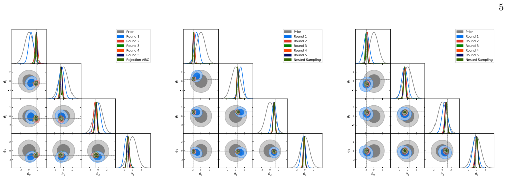
The first figure displays the prior and rounds 1 and 2, while the second shows rounds 3 to 5; in both cases the nested sampling result is shown. It can be noted by eye that the posterior coincides well with the result of nested sampling after four to five rounds of LSBI. This suggests that, although the CMB power spectrum is not well approximated by a lin...

work page
[8]

A. Cole, B. K. Miller, S. J. Witte, M. X. Cai, M. W. Grootes, F. Nattino, and C. Weniger, Fast and credible likelihood-free cosmology with truncated marginal neural ratio estimation, Journal of Cosmology and Astroparticle Physics 2022 (09), 004

work page 2022

Show all 31 references

[9]

Lemos, M

P. Lemos, M. Cranmer, M. Abidi, C. Hahn, M. Eick- enberg, E. Massara, D. Yallup, and S. Ho, Robust simulation-based inference in cosmology with bayesian neural networks, Machine Learning: Science and Tech- nology 4, 01LT01 (2023)

2023
[10]

Papamakarios, Neural density estimation and likelihood-free inference, arXiv preprint arXiv:1910.13233 (2019)

G. Papamakarios, Neural density estimation and likelihood-free inference, arXiv preprint arXiv:1910.13233 (2019)

2019 arXiv
[11]

Dupourqu´ e, N

S. Dupourqu´ e, N. Clerc, E. Pointecouteau, D. Eckert, S. Ettori, and F. Vazza, Investigating the turbulent hot gas in x-cop galaxy clusters, Astronomy & Astrophysics 673, A91 (2023)

2023
[12]

Gatti, N

M. Gatti, N. Jeffrey, L. Whiteway, J. Williamson, B. Jain, V. Ajani, D. Anbajagane, G. Giannini, C. Zhou, A. Porredon, et al., Dark energy survey year 3 results: Simulation-based cosmological inference with wavelet harmonics, scattering transforms, and moments of weak lensing ...

2024
[13]

Crisostomi, K

M. Crisostomi, K. Dey, E. Barausse, and R. Trotta, Neural posterior estimation with guaranteed exact cover- age: The ringdown of gw150914, Physical Review D 108, 044029 (2023)

2023
[14]

Christy, E

K. Christy, E. J. Baxter, and J. Kumar, Applying simulation-based inference to spectral and spatial infor- mation from the galactic center gamma-ray excess, arXiv preprint arXiv:2402.04549 (2024)

2024 arXiv
[15]

Harnois-Deraps, S

J. Harnois-Deraps, S. Heydenreich, B. Giblin, N. Mar- tinet, T. Troester, M. Asgari, P. Burger, T. Castro, K. Dolag, C. Heymans, et al., Kids-1000 and des-y1 combined: Cosmology from peak count statistics, arXiv preprint arXiv:2405.10312 (2024)

2024 arXiv
[16]

Moser, T

B. Moser, T. Kacprzak, S. Fischbacher, A. Refregier, D. Grimm, and L. Tortorelli, Simulation-based inference of deep fields: galaxy population model and redshift distributions, Journal of Cosmology and Astroparticle Physics 2024 (05), 049

2024
[17]

C. P. Novaes, L. Thiele, J. Armijo, S. Cheng, J. A. Cow- ell, G. A. Marques, E. G. Ferreira, M. Shirasaki, K. Os- ato, and J. Liu, Cosmology from hsc y1 weak lensing with combined higher-order statistics and simulation-based in- ference, arXiv preprint arXiv:2409.01301 (2024)

2024 arXiv
[18]

Fischbacher, B

S. Fischbacher, B. Moser, T. Kacprzak, J. Herbel, L. Tor- torelli, U. Schmitt, A. Refregier, and A. Amara, galsbi : A python package for the galsbi galaxy population model, arXiv preprint arXiv:2412.08722 (2024)

2024
[19]

Castelvecchi, Can we open the black box of ai?, Nature News 538, 20 (2016)

D. Castelvecchi, Can we open the black box of ai?, Nature News 538, 20 (2016)

2016
[20]

Hermans, A

J. Hermans, A. Delaunoy, F. Rozet, A. Wehenkel, V. Begy, and G. Louppe, A trust crisis in simulation- based inference? your posterior approximations can be unfaithful, arXiv preprint arXiv:2110.06581 (2021)

2021 arXiv
[21]

Leclercq, W

F. Leclercq, W. Enzi, J. Jasche, and A. Heavens, Pri- mordial power spectrum and cosmology from black-box galaxy surveys, Monthly Notices of the Royal Astronom- ical Society 490, 4237 (2019)

2019
[22]

A. F. Heavens, R. Jimenez, and O. Lahav, Massive loss- less data compression and multiple parameter estimation from galaxy spectra, Monthly Notices of the Royal As- tronomical Society 317, 965 (2000)

2000
[23]

A. K. Gupta and D. K. Nagar, Matrix variate distribu- tions (Chapman and Hall/CRC, 2018)

2018
[24]

Piras and A

D. Piras and A. S. Mancini, Cosmopower-jax: high- dimensional bayesian inference with differentiable cos- mological emulators, arXiv preprint arXiv:2305.06347 (2023)

2023 arXiv
[25]

Spurio Mancini, D

A. Spurio Mancini, D. Piras, J. Alsing, B. Joachimi, and M. P. Hobson, Cosmopower: emulating cosmologi- cal power spectra for accelerated bayesian inference from next-generation surveys, Monthly Notices of the Royal Astronomical Society 511, 1771 (2022)

2022
[26]

J. S. Speagle, dynesty: a dynamic nested sampling pack- age for estimating bayesian posteriors and evidences, Monthly Notices of the Royal Astronomical Society 493, 3132 (2020)

2020
[27]

Koposov, J

S. Koposov, J. Speagle, K. Barbary, G. Ashton, E. Ben- nett, J. Buchner, C. Scheffler, B. Cook, C. Talbot, J. Guillochon, et al., joshspeagle/dynesty: v2. 0.0, Zen- odo (2022)

2022
[28]

Higson, W

E. Higson, W. Handley, M. Hobson, and A. Lasenby, Dy- namic nested sampling: an improved algorithm for pa- rameter estimation and evidence calculation, Statistics and Computing 29, 891 (2019)

2019
[29]

Lewis, Getdist: a python package for analysing monte carlo samples, arXiv preprint arXiv:1910.13970 (2019)

A. Lewis, Getdist: a python package for analysing monte carlo samples, arXiv preprint arXiv:1910.13970 (2019)

2019 arXiv
[30]

Alsing and B

J. Alsing and B. Wandelt, Generalized massive optimal data compression, Monthly Notices of the Royal Astro- nomical Society: Letters 476, L60 (2018)

2018
[31]

Alsing, B

J. Alsing, B. Wandelt, and S. Feeney, Massive optimal data compression and density estimation for scalable, likelihood-free inference in cosmology, Monthly Notices of the Royal Astronomical Society 477, 2874 (2018)

2018

Pith tools

Reviewed August 10, 2026 · model on record in the stance chip above.

[1] [1]

Cranmer, J

K. Cranmer, J. Brehmer, and G. Louppe, The frontier of simulation-based inference, Proceedings of the National Academy of Sciences 117, 30055 (2020)

2020

[2] [2]

D. B. Rubin, Bayesianly justifiable and relevant fre- quency calculations for the applied statistician, The An- nals of Statistics , 1151 (1984)

work page 1984

[3] [3]

Marjoram, J

P. Marjoram, J. Molitor, V. Plagnol, and S. Tavar´ e, Markov chain monte carlo without likelihoods, Proceed- ings of the National Academy of Sciences 100, 15324 (2003)

work page 2003

[4] [4]

S. A. Sisson, Y. Fan, and M. M. Tanaka, Sequential monte carlo without likelihoods, Proceedings of the Na- tional Academy of Sciences 104, 1760 (2007)

work page 2007

[5] [5]

Papamakarios and I

G. Papamakarios and I. Murray, Fast ε-free inference of simulation models with bayesian conditional density es- timation, Advances in neural information processing sys- tems 29 (2016)

work page 2016

[6] [6]

Alsing, T

J. Alsing, T. Charnock, S. Feeney, and B. Wandelt, Fast likelihood-free cosmology with neural density estimators and active learning, Monthly Notices of the Royal Astro- nomical Society 488, 4440 (2019)

work page 2019

[7] [7]

It can be noted by eye that the posterior coincides well with the result of nested sampling after four to five rounds of LSBI

The first figure displays the prior and rounds 1 and 2, while the second shows rounds 3 to 5; in both cases the nested sampling result is shown. It can be noted by eye that the posterior coincides well with the result of nested sampling after four to five rounds of LSBI. This suggests that, although the CMB power spectrum is not well approximated by a lin...

work page

[8] [8]

A. Cole, B. K. Miller, S. J. Witte, M. X. Cai, M. W. Grootes, F. Nattino, and C. Weniger, Fast and credible likelihood-free cosmology with truncated marginal neural ratio estimation, Journal of Cosmology and Astroparticle Physics 2022 (09), 004

work page 2022