Generalized Functional ANOVA in Closed-Form: A Unified View of Additive Explanations
Pith reviewed 2026-05-19 23:53 UTC · model grok-4.3
The pith
Hilbert space methods yield an explicit Riesz basis for generalized functional ANOVA on continuous dependent inputs
A machine-rendered reading of the paper's core claim, the machinery that carries it, and where it could break.
Core claim
By combining Hilbert space methods with the generalized functional ANOVA, we build an explicit decomposition Riesz Basis allowing to easily compute the decomposition. Our formulation recovers the classical independent case and its associated orthogonal decomposition. Building on this representation, we propose a simple but mighty algorithm to estimate the decomposition from a data sample in a model-agnostic setting and we compare it empirically with several state-of-the-art explanation methods, demonstrating the power of the approach.
What carries the argument
the explicit decomposition Riesz Basis constructed in the Hilbert space of the input measure, which represents every term of the generalized functional ANOVA as an inner product against basis elements
If this is right
- The decomposition can be evaluated in closed form once the basis coefficients are known, without numerical integration over the joint distribution.
- The independent-input orthogonal ANOVA appears as the special case in which the Riesz basis reduces to the usual product basis.
- A model-agnostic estimator follows immediately by replacing population inner products with their empirical counterparts on a sample.
- The same representation connects the decomposition to SHAP values and to the terms of a generalized additive model.
Where Pith is reading between the lines
- Choosing particular Riesz bases, such as orthogonal polynomials with respect to the marginal measures, could yield fast algorithms that scale to moderate dimensions.
- The construction supplies a theoretical justification for applying additive explanation methods to correlated features without first transforming the data to independence.
- If the Riesz basis can be adapted to mixed continuous-discrete inputs, the same closed-form route would extend to a wider class of tabular data problems.
Load-bearing premise
The input variables are continuous and the underlying Hilbert space admits a suitable Riesz basis so that the decomposition stays explicit and can be estimated from finite samples.
What would settle it
Generate synthetic continuous data with known dependence structure, compute the true generalized functional ANOVA terms by direct integration, then apply the proposed estimator and check whether the recovered terms match the true decomposition to within sampling error.
Figures


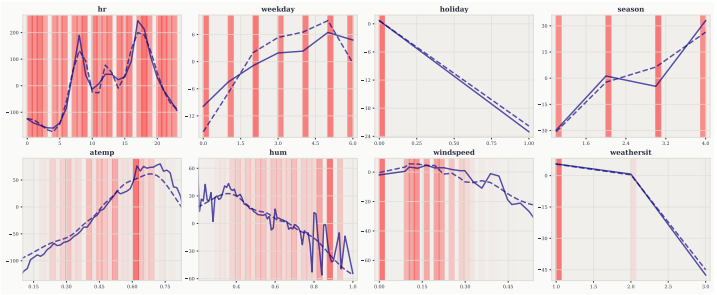
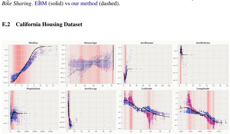
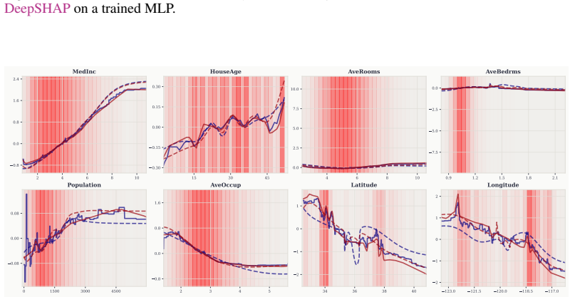


read the original abstract
The functional ANOVA, or Hoeffding decomposition, provides a principled framework for interpretability by decomposing a model prediction into main effects and higher-order interactions. For independent inputs, this classical decomposition is explicit. It is closely connected to SHAP values, generalized additive models, and orthogonal polynomial expansions, and therefore constitutes a fundamental tool for additive explainability. In the more general and realistic dependent setting, however, obtaining a tractable representation and estimating the decomposition from data remain challenging. In this work, we address this problem for continuous inputs. By combining Hilbert space methods with the generalized functional ANOVA, we build an explicit decomposition Riesz Basis allowing to easily compute the decomposition. Our formulation recovers the classical independent case and its associated orthogonal decomposition. Building on this representation, we propose a simple but mighty algorithm to estimate the decomposition from a data sample in a model-agnostic setting and we compare it empirically with several state-of-the-art explanation methods, demonstrating the power of the approach.
Editorial analysis
A structured set of objections, weighed in public.
Referee Report
Summary. The manuscript claims that Hilbert-space methods applied to the generalized functional ANOVA yield an explicit Riesz basis for decomposing model predictions into additive terms and interactions when inputs are continuous and possibly dependent. The resulting representation is asserted to be directly computable, to recover the classical orthogonal Hoeffding decomposition under independence, and to support a simple model-agnostic estimation procedure from finite samples whose performance is compared empirically with existing explanation methods.
Significance. If the explicit Riesz-basis construction is valid and remains tractable for general joint distributions, the work would supply a principled, closed-form unification of additive explanations that extends beyond the independent-input case while preserving connections to SHAP, GAMs, and orthogonal expansions. The empirical comparisons constitute a concrete strength that would help establish practical utility.
major comments (2)
- [Abstract and Riesz-basis construction section] Abstract and the section presenting the Riesz-basis construction: the central claim that an explicit, easily computable Riesz basis exists for arbitrary continuous joint distributions is load-bearing, yet the provided outline supplies neither the explicit form of the basis functions nor a demonstration that coefficient extraction avoids solving a Fredholm integral equation whose kernel depends on the unknown density; without this, the 'closed-form' and 'easily compute' guarantees cannot be verified.
- [Recovery of independent case] Section on recovery of the independent case: the manuscript must show, via direct substitution or limit argument, that the generalized basis reduces exactly to the classical orthogonal decomposition when the joint measure factors, rather than merely stating recovery at a high level.
minor comments (2)
- [Preliminaries] Clarify the precise definition of the underlying Hilbert space L²(μ) and the inner product used to define the Riesz basis, including any regularity conditions on the joint density.
- [Experiments] The empirical section would benefit from reporting standard errors or confidence intervals on the explanation metrics to strengthen the comparison with state-of-the-art methods.
Simulated Author's Rebuttal
We thank the referee for their constructive and detailed comments. These have helped us identify areas where the manuscript would benefit from greater explicitness and rigor. We address each major comment below and have revised the manuscript to incorporate the requested details, proofs, and clarifications.
read point-by-point responses
-
Referee: [Abstract and Riesz-basis construction section] Abstract and the section presenting the Riesz-basis construction: the central claim that an explicit, easily computable Riesz basis exists for arbitrary continuous joint distributions is load-bearing, yet the provided outline supplies neither the explicit form of the basis functions nor a demonstration that coefficient extraction avoids solving a Fredholm integral equation whose kernel depends on the unknown density; without this, the 'closed-form' and 'easily compute' guarantees cannot be verified.
Authors: We agree that the original presentation would be strengthened by a more detailed derivation of the Riesz basis. In the revised manuscript we now include an explicit construction: the basis functions are the Riesz representers of the coordinate functionals on the subspaces of the generalized ANOVA decomposition with respect to the joint measure. These are obtained via a Gram-Schmidt orthogonalization that exploits the nested structure of the ANOVA subspaces, yielding closed-form expressions involving only the joint density evaluated at the observed points and the marginal conditionals. We further show that the expansion coefficients are inner products that reduce to expectations under the data-generating distribution; these expectations are estimated directly from samples via Monte Carlo averages and do not require solving any integral equation whose kernel involves the unknown density. A new subsection with the full derivation and a worked example for the bivariate case has been added. revision: yes
-
Referee: [Recovery of independent case] Section on recovery of the independent case: the manuscript must show, via direct substitution or limit argument, that the generalized basis reduces exactly to the classical orthogonal decomposition when the joint measure factors, rather than merely stating recovery at a high level.
Authors: We thank the referee for this precise request. The revised manuscript now contains a dedicated lemma with a direct substitution argument. When the joint measure factors as the product of the marginals, the inner-product structure of the generalized Riesz basis collapses to the standard L² inner product with respect to the product measure. Substituting the product form into the defining equations for the basis functions shows that they coincide exactly with the classical orthogonal polynomials (or indicator functions) of the Hoeffding decomposition. The coefficients likewise reduce to the usual centered conditional expectations. The proof is presented in full, including the verification that all cross terms vanish under independence. revision: yes
Circularity Check
Derivation is a direct Hilbert-space construction with no reduction to inputs by construction
full rationale
The paper constructs an explicit Riesz basis for the generalized functional ANOVA by combining standard Hilbert-space methods with the existing generalized ANOVA framework for continuous inputs. The abstract states that this yields a tractable decomposition that recovers the classical orthogonal Hoeffding decomposition under independence, which functions as a consistency check rather than an input. No equations or steps are shown that define a quantity in terms of itself, rename a fitted parameter as a prediction, or rely on a load-bearing self-citation whose content is unverified. The central claim remains a mathematical construction from external functional-analysis results and is therefore self-contained.
Axiom & Free-Parameter Ledger
axioms (1)
- domain assumption Input variables are continuous.
invented entities (1)
-
Riesz basis for the generalized functional ANOVA
no independent evidence
Lean theorems connected to this paper
-
IndisputableMonolith/Foundation/RealityFromDistinction.leanreality_from_one_distinction unclear?
unclearRelation between the paper passage and the cited Recognition theorem.
By combining Hilbert space methods with the generalized functional ANOVA, we build an explicit decomposition Riesz Basis... recovers the classical independent case and its associated orthogonal decomposition.
-
IndisputableMonolith/Cost/FunctionalEquation.leanwashburn_uniqueness_aczel unclear?
unclearRelation between the paper passage and the cited Recognition theorem.
ξ(m_S)_S(x) := 1/√(2^{p−|S|}) · ∏_{j∈S} eP_{m_j}(x_j) / f_S(x_S)
What do these tags mean?
- matches
- The paper's claim is directly supported by a theorem in the formal canon.
- supports
- The theorem supports part of the paper's argument, but the paper may add assumptions or extra steps.
- extends
- The paper goes beyond the formal theorem; the theorem is a base layer rather than the whole result.
- uses
- The paper appears to rely on the theorem as machinery.
- contradicts
- The paper's claim conflicts with a theorem or certificate in the canon.
- unclear
- Pith found a possible connection, but the passage is too broad, indirect, or ambiguous to say the theorem truly supports the claim.
Reference graph
Works this paper leans on
-
[1]
Agarwal, R., Melnick, L., Frosst, N., Zhang, X., Lengerich, B., Caruana, R., and Hinton, G. E. (2021). Neural additive models: Interpretable machine learning with neural nets.Advances in neural information processing systems, 34:4699–4711
work page 2021
-
[2]
Amoukou, S. I., Salaün, T., and Brunel, N. (2022). Accurate Shapley values for explaining tree-based models. InInternational conference on artificial intelligence and statistics, pages 2448–2465. PMLR
work page 2022
-
[3]
Apley, D. W. and Zhu, J. (2020). Visualizing the effects of predictor variables in black box super- vised learning models.Journal of the Royal Statistical Society Series B: Statistical Methodology, 82(4):1059–1086
work page 2020
-
[4]
Arzamasov, V ., Böhm, K., and Jochem, P. (2018). Towards concise models of grid stability. In 2018 IEEE international conference on communications, control, and computing technologies for smart grids (SmartGridComm), pages 1–6. IEEE
work page 2018
-
[5]
Bach, S., Binder, A., Montavon, G., Klauschen, F., Müller, K.-R., and Samek, W. (2015). On pixel-wise explanations for non-linear classifier decisions by layer-wise relevance propagation. PloS one, 10(7):e0130140
work page 2015
-
[6]
Bénard, C. (2025). Tree Ensemble Explainability through the Hoeffding Functional Decomposi- tion and TreeHFD Algorithm.Advances in Neural Information Processing Systems
work page 2025
-
[7]
Blatman, G. and Sudret, B. (2011). Adaptive sparse polynomial chaos expansion based on least angle regression.Journal of computational Physics, 230(6):2345–2367
work page 2011
-
[8]
Bordt, S. and von Luxburg, U. (2023). From Shapley values to generalized additive models and back. InInternational Conference on Artificial Intelligence and Statistics, pages 709–745. PMLR
work page 2023
-
[9]
(2011).Functional analysis, Sobolev spaces and partial differential equations, volume 2
Brézis, H. (2011).Functional analysis, Sobolev spaces and partial differential equations, volume 2. Springer
work page 2011
-
[10]
Cencov, N. N. (1962). Estimation of an unknown distribution density from observations.Soviet Math., 3:1559–1566
work page 1962
- [11]
-
[12]
Chastaing, G., Gamboa, F., and Prieur, C. (2012). Generalized Hoeffding-Sobol Decomposition for Dependent Variables – Application to Sensitivity Analysis.Electronic Journal of Statistics, 6:2420–2448
work page 2012
-
[13]
Chen, T., He, T., Benesty, M., Khotilovich, V ., Tang, Y ., Cho, H., Chen, K., Mitchell, R., Cano, I., Zhou, T., et al. (2015). Xgboost: extreme gradient boosting.R package version 0.4-2, 1(4):1–4
work page 2015
-
[14]
Courant, R. and Hilbert, D. (2024).Methods of mathematical physics, volume 2. John Wiley & Sons
work page 2024
-
[15]
Dua, D., Graff, C., et al. (2017). Uci machine learning repository, 2017.URL http://archive. ics. uci. edu/ml, 7(1):62
work page 2017
-
[16]
Efron, B., Hastie, T., Johnstone, I., and Tibshirani, R. (2004). Least angle regression.The Annals of Statistics, 32(2). 10
work page 2004
-
[17]
Fanaee-T, H. and Gama, J. (2014). Event labeling combining ensemble detectors and background knowledge.Progress in Artificial Intelligence, 2(2):113–127
work page 2014
- [18]
-
[19]
Ghanem, R. G. and Spanos, P. D. (2003).Stochastic finite elements: a spectral approach. Courier Corporation
work page 2003
-
[20]
Hamidieh, K. (2018). A data-driven statistical model for predicting the critical temperature of a superconductor.Computational Materials Science, 154:346–354
work page 2018
-
[21]
Harris, C. R., Millman, K. J., Van Der Walt, S. J., Gommers, R., Virtanen, P., Cournapeau, D., Wieser, E., Taylor, J., Berg, S., Smith, N. J., et al. (2020). Array programming with NumPy. Nature, 585(7825):357–362
work page 2020
-
[22]
Harsanyi, J. C. (1963). A Simplified Bargaining Model for the n−Person Cooperative Game. International Economic Review, 4(2):194–220
work page 1963
-
[23]
Hastie, T. J. (2017). Generalized additive models. InStatistical models in S, pages 249–307. Routledge
work page 2017
-
[24]
Herren, A. and Hahn, P. R. (2022). Statistical aspects of SHAP: Functional ANOV A for model interpretation.arXiv:2208.09970
-
[25]
Hiabu, M., Meyer, J. T., and Wright, M. N. (2023). Unifying local and global model explanations by functional decomposition of low dimensional structures. InInternational conference on artificial intelligence and statistics, pages 7040–7060. PMLR
work page 2023
-
[26]
Hoeffding, W. (1948). A Class of Statistics with Asymptotically Normal Distribution.The Annals of Mathematical Statistics, 19(3):293–325
work page 1948
-
[27]
Hooker, G. (2007). Generalized Functional ANOV A Diagnostics for High-Dimensional Func- tions of Dependent Variables.Journal of Computational and Graphical Statistics, 16(3):709–732
work page 2007
-
[28]
I., Bousquet, N., Gamboa, F., Iooss, B., and Loubes, J.-M
Idrissi, M. I., Bousquet, N., Gamboa, F., Iooss, B., and Loubes, J.-M. (2025). Hoeffding decomposition of functions of random dependent variables.Journal of Multivariate Analysis, 208:105444
work page 2025
-
[29]
Kingma, D. P. and Ba, J. (2014). Adam: A method for stochastic optimization.arXiv preprint arXiv:1412.6980
work page internal anchor Pith review Pith/arXiv arXiv 2014
-
[30]
Kohavi, R. et al. (1996). Scaling up the accuracy of naive-Bayes classifiers: A decision-tree hybrid. InKdd, volume 96, pages 202–207
work page 1996
-
[31]
E., Venkatasubramanian, S., Scheidegger, C., and Friedler, S
Kumar, I. E., Venkatasubramanian, S., Scheidegger, C., and Friedler, S. (2020). Problems with Shapley-value-based explanations as feature importance measures. InInternational conference on machine learning, pages 5491–5500. PMLR
work page 2020
-
[32]
Lengerich, B., Tan, S., Chang, C.-H., Hooker, G., and Caruana, R. (2020). Purifying interaction effects with the functional ANOV A: An efficient algorithm for recovering identifiable additive models. InInternational Conference on Artificial Intelligence and Statistics, pages 2402–2412. PMLR
work page 2020
-
[33]
Lipovetsky, S. and Conklin, M. (2001). Analysis of regression in game theory approach.Applied stochastic models in business and industry, 17(4):319–330
work page 2001
-
[34]
Lou, Y ., Caruana, R., Gehrke, J., and Hooker, G. (2013). Accurate intelligible models with pairwise interactions. InProceedings of the 19th ACM SIGKDD international conference on Knowledge Discovery and Data mining, pages 623–631
work page 2013
-
[35]
Consistent Individualized Feature Attribution for Tree Ensembles
Lundberg, S. M., Erion, G. G., and Lee, S.-I. (2018). Consistent individualized feature attribution for tree ensembles.arXiv:1802.03888. 11
work page internal anchor Pith review Pith/arXiv arXiv 2018
-
[36]
Lundberg, S. M. and Lee, S.-I. (2017). A unified approach to interpreting model predictions. Advances in neural information processing systems, 30
work page 2017
-
[37]
Montgomery, D. C. (2017).Design and analysis of experiments. John Wiley & Sons
work page 2017
-
[38]
Muschalik, M., Baniecki, H., Fumagalli, F., Kolpaczki, P., Hammer, B., and Hüllermeier, E. (2024a). shapiq: Shapley interactions for machine learning.Advances in Neural Information Processing Systems, 37:130324–130357
-
[39]
Muschalik, M., Fumagalli, F., Hammer, B., and Hüllermeier, E. (2024b). Beyond TreeSHAP: Efficient computation of any-order shapley interactions for tree ensembles. InProceedings of the AAAI Conference on Artificial Intelligence, volume 38, pages 14388–14396
-
[40]
Nelsen, R. B. (2006).An introduction to copulas. Springer
work page 2006
- [41]
-
[42]
Owen, A. B. (2014). Sobol’indices and Shapley value.SIAM/ASA Journal on Uncertainty Quantification, 2(1):245–251
work page 2014
-
[43]
Owen, A. B. and Prieur, C. (2017). On Shapley value for measuring importance of dependent inputs.SIAM/ASA Journal on Uncertainty Quantification, 5(1):986–1002
work page 2017
-
[44]
Pace, R. K. and Barry, R. (1997). Sparse spatial autoregressions.Statistics & Probability Letters, 33(3):291–297
work page 1997
-
[45]
Pedregosa, F., Varoquaux, G., Gramfort, A., Michel, V ., Thirion, B., Grisel, O., Blondel, M., Prettenhofer, P., Weiss, R., Dubourg, V ., et al. (2011). Scikit-learn: Machine learning in Python. Journal of Machine Learning Research, 12:2825–2830
work page 2011
- [46]
-
[47]
Radenovic, F., Dubey, A., and Mahajan, D. (2022). Neural basis models for interpretability. Advances in Neural Information Processing Systems, 35:8414–8426
work page 2022
-
[48]
Rahman, S. (2014). A generalized ANOV A dimensional decomposition for dependent probabil- ity measures.SIAM/ASA Journal on Uncertainty Quantification, 2(1):670–697
work page 2014
-
[49]
Reed, M. and Simon, B. (1980). V olume 1: Functional analysis. InMethods of Modern Mathematical Physics. Elsevier
work page 1980
-
[50]
Ribeiro, M. T., Singh, S., and Guestrin, C. (2016). " Why should I trust you?" Explaining the predictions of any classifier. InProceedings of the 22nd ACM SIGKDD international conference on Knowledge Discovery and Data mining, pages 1135–1144
work page 2016
-
[51]
Rota, G.-C. (1964). On the foundations of combinatorial theory: I. theory of Möbius functions. InClassic Papers in Combinatorics, pages 332–360. Springer
work page 1964
-
[52]
Shapley, L. S. (1953).A Value for n-Person Games, pages 307–318. Princeton University Press, Princeton
work page 1953
-
[53]
Shrikumar, A., Greenside, P., and Kundaje, A. (2017). Learning important features through propagating activation differences. InInternational Conference on Machine Learning, pages 3145–3153. PMLR
work page 2017
-
[54]
Smith, J. W., Everhart, J. E., Dickson, W. C., Knowler, W. C., and Johannes, R. S. (1988). Using the adap learning algorithm to forecast the onset of diabetes mellitus. InProceedings of the Annual Symposium on Computer Application in Medical Care, page 261
work page 1988
-
[55]
Stone, C. J. (1994). The use of polynomial splines and their tensor products in multivariate function estimation.The Annals of Statistics, pages 118–171. 12
work page 1994
-
[56]
Sundararajan, M. and Najmi, A. (2020). The many Shapley values for model explanation. In International Conference on Machine Learning, pages 9269–9278. PMLR
work page 2020
-
[57]
(1939).Orthogonal polynomials, volume 23
Szeg ˝o, G. (1939).Orthogonal polynomials, volume 23. American Mathematical Soc
work page 1939
-
[58]
(2008).Spectral theory of block operator matrices and applications
Tretter, C. (2008).Spectral theory of block operator matrices and applications. World Scientific
work page 2008
-
[59]
Virtanen, P., Gommers, R., Oliphant, T. E., Haberland, M., Reddy, T., Cournapeau, D., Burovski, E., Peterson, P., Weckesser, W., Bright, J., et al. (2020). Scipy 1.0: fundamental algorithms for scientific computing in python.Nature methods, 17(3):261–272
work page 2020
-
[60]
Xiu, D. and Karniadakis, G. E. (2002). The Wiener–Askey polynomial chaos for stochastic differential equations.SIAM Journal on Scientific Computing, 24(2):619–644
work page 2002
-
[61]
Yang, Z., Zhang, A., and Sudjianto, A. (2021). GAMI-Net: An explainable neural network based on generalized additive models with structured interactions.Pattern Recognition, 120:108192
work page 2021
-
[62]
1√ 2p−|S| Y s∈S ePms(Xs) fs(Xs) · 1√ 2p−|T| Y t∈T ePnt(Xt) ft(Xt) # (70) ∝E
Yu, G., Bien, J., and Tibshirani, R. (2019). Reluctant interaction modeling.arXiv:1907.08414. 13 A Legendre Polynomials In this section, we rely on results that have been widely studied by [57]. Definition A.1.For any non-negative integer m∈N , we denote by Pm the Legendre polynomial of degreem. This family is uniquely defined by the three-term recurrence...
discussion (0)
Sign in with ORCID, Apple, or X to comment. Anyone can read and Pith papers without signing in.