REVIEW 3 major objections 8 minor 15 references
Review of Algorithms for Compressive Sensing of Images
T0 review · 3 major / 8 minor · reviewed 2026-08-14 · deepseek-v4-flash
Pith's one-line read The paper claims that total variation minimization reconstructs natural images better than L1 minimization on a sparsifying basis, with NESTA and TVAL3 as the most practical algorithms.
desk verdict Readable tutorial with a useful noise comparison, but the headline L1-vs-TV conclusion is confounded by different forward models and measurement rates. read the letter →
The pith
A machine-rendered reading of the paper's core claim, the machinery that carries it, and where it could break.
The reading
What carries the argument
The load-bearing mechanism is the total variation pseudo-norm, the L1 norm of the discrete gradient, which is nearly sparse for natural images and keeps reconstruction errors local instead of producing global interference patterns. NESTA works by applying Nesterov's accelerated gradient method with smoothing to reach a $\mathcal{O}(1/k^2)$ convergence rate, which is what preserves image features under noise. TVAL3 works by minimizing an augmented Lagrangian with an alternating-direction non-monotone line search, which is what makes it fast. Both solvers rely only on matrix-vector products, so they can exploit fast measurement bases such as the Dragon wavelet group, computed in $O(n\log n)$ time.
What would settle it
Run the same image and SNR comparison with physically realizable measurements, such as random pixel masks on a digital micromirror device, instead of pre-computed transform coefficients; if L1-on-wavelets then matches or beats total variation, the paper's central conclusion is unsupported.
Extended reading notes
Core claim
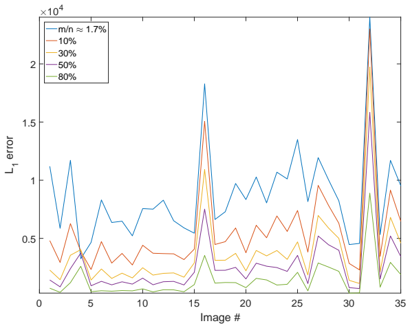
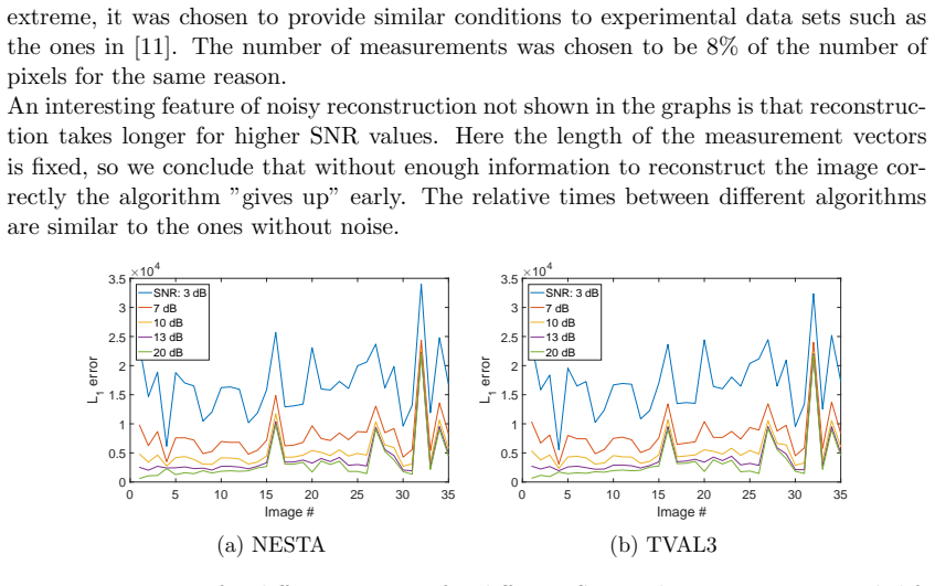
The central discovery is that TV-regularized reconstruction of natural images needs far fewer measurements than L1 reconstruction on sparsified coefficients and produces visually better results at comparable L1 error. This is supported by controlled runs of L1 Magic, NESTA, TVAL3, GPSR, and SPGL1 on 35 images, with measurement ratios from about 0.17% to 80% and signal-to-noise ratios from 3 dB to 20 dB. In the noisy regime relevant to LiDAR, NESTA preserves overall structure at low SNR while TVAL3 fails; at high SNR, TVAL3 reconstructs roughly three times faster than NESTA and about ten times faster than L1 Magic. The paper therefore concludes that TV is more appropriate than L1 under a sparsifying basis and that the practical choice is between NESTA for noise tolerance and TVAL3 for speed.
Load-bearing premise
The L1-versus-TV comparison assumes a sensing system can directly measure the sparse transform coefficients $z=\varphi x$; if a real camera cannot, the L1 experiments do not test a usable reconstruction method.
Editorial extensions
If this is right
- For natural-image compressive sensing, a total-variation solver should be preferred over an L1 solver applied to sparsified coefficients.
- In low-SNR measurement settings, NESTA is the safer default because its output retains major image structure that post-processing can improve.
- In well-conditioned high-SNR settings, TVAL3 is the faster default, roughly three times faster than NESTA and ten times faster than L1 Magic.
- Reconstruction succeeds with a small percentage of measurements, but quality degrades sharply near the information limit and at low SNR.
- Image content matters as much as algorithm choice: noise-like images and images with sharp edges reconstruct with higher error under every method.
Reading between the lines
- A physically realizable sensor cannot measure transform coefficients directly, so the L1 comparison in this paper is a simulation convenience; a hardware test may show an even larger gap in favor of TV because the L1 route may not be implementable at all.
- NESTA's low-SNR tolerance makes it a natural starting point for photon-starved imaging where each measurement is expensive; the noise model was chosen to match such data, so testing on the author's LiDAR setup is a direct next step.
- The relative ranking of NESTA and TVAL3 could shift under a different sampling basis, since the paper never quantifies the choice of Dragon wavelets against alternatives such as scrambled Hadamard vectors.
Signed reviews
Editorial analysis
A structured set of objections, weighed in public.
Referee Report
Summary. This manuscript is a tutorial-style review of classical compressive sensing algorithms for images, with emphasis on total variation (TV) methods and a target application to LiDAR. It introduces basic CS theory, reviews L1-based solvers (OMP, LASSO, GPSR, SPGL1, L1 Magic, NESTA) and TV-based solvers (L1 Magic TV, NESTA, TVAL3), and reports simulation comparisons of runtime and reconstruction error across measurement ratios and noise levels. Its headline conclusions are that TV minimization is more appropriate than L1 minimization for natural images and that NESTA and TVAL3 are the most practical algorithms.
Significance. A reliable practical comparison of off-the-shelf CS solvers would be valuable to practitioners, and the paper makes a reasonable effort to treat algorithms as black boxes, to include noisy measurements, and to provide its code. However, the experimental design confounds the regularizer with the forward operator and the measurement schedule, so the main comparative claim is not established. Because the paper's primary contribution is the practical recommendation, its significance depends entirely on correcting this flaw.
major comments (3)
- [2.4, 3, 5] The comparison that drives the paper's central conclusion is confounded. The L1 experiments reconstruct z = Φx from measurements y = Ψz, i.e., y = ΨΦx, with z computed by a pre-step that the author states 'is not applicable to a real-world system' (§2.4). The TV experiments instead reconstruct x from y = Ψx (§3). Thus the L1 and TV solvers are given different forward operators, and the observed advantage of TV could be an artifact of the sensing matrix or of oracle access to the sparse coefficients rather than of the regularizer. Since §5's first conclusion is that TV is more appropriate than L1 for natural images, this load-bearing comparison must be redone with identical sensing matrices and without oracle access to the sparse coefficients.
- [3.4.1, Figs. 2 and 5] The measurement-ratio schedules differ between the two algorithm classes. L1 results are shown at m/n = 1.7%, 10%, 30%, 50%, 80% (Fig. 2), while TV results are shown at m/n = 0.17%, 1%, 1.7%, 10%, 30% (Fig. 5). The claim that TV needs a smaller percentage of measurements is not established by this comparison, because the two classes are not evaluated on the same ratios; a matched comparison at common ratios (e.g., 1.7%, 10%, 30%) with the same sensing operator is required before drawing that conclusion.
- [2.4, 3.4, 4] The experimental protocol omits key details needed to judge the comparison. The 'L1 error' metric is not defined; the tuning parameters (τ, σ, λ, μ) for each algorithm are not reported; no error bars or multiple noise realizations are shown in Figure 7; and the image dimensions are not stated. Because the paper's value is a practical 'which algorithm should I use' guide, these omissions make the runtime and quality comparisons irreproducible and potentially non-representative. The author should provide a complete protocol, including parameter values and a direct link to the code.
minor comments (8)
- [Eq. (1)] In Eq. (1), the approximation −(k/n) log(k/n) − (1−k/n) log(1−k/n) ≈ (k/n) log(k/n) is incorrect in sign; the entropy of the sparse Bernoulli source is positive and behaves as (k/n) log(n/k) for small k/n. The error propagates into the intuitive bound that follows.
- [Eq. (4)] In Eq. (4), the constraint y_k = (φ x')_k is inconsistent with the model in §2, where measurements are taken in the sampling basis ψ (i.e., y = ψ x); the sparsifying basis φ should appear in the objective, not in the measurement constraint. This is a significant clarity issue in a review intended for beginners.
- [3.2] The heading 'Nestorov's algorithm' should read 'Nesterov's algorithm' to match the reference to Nesterov in the bibliography.
- [2.4] The phrase 'compression ration' should be 'compression ratio'.
- [3.3] The phrase 'the algorithms inability' should be 'the algorithm's inability'.
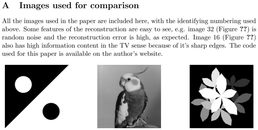
- [Appendix A] Several figure cross-references appear as 'Figure ??', and the image dimensions are not given, which prevents quantitative interpretation of the reported m/n ratios and runtimes.
- [A] The code availability statement says the code is on the author's website but provides no URL; a persistent repository link is needed for reproducibility.
- [1.1] The sentence 'the measurement basis in incoherent with the basis' should read 'the measurement basis is incoherent with the basis'.
Circularity Check
No significant circularity: the paper's comparative conclusions rest on its own simulations, not on a reduction to inputs or on load-bearing self-citation.
full rationale
This paper is a review and experimental comparison of off-the-shelf compressive-sensing algorithms. Its central claims—that total-variation minimization is more appropriate than L1 minimization for natural images and that NESTA and TVAL3 stand out—are supported by the simulation results in Sections 2.4, 3.4, and 4, not by a derivation from the assumptions. The self-citations are not load-bearing: reference [11] motivates the noise settings in Section 4, and reference [5] supplies the Dragon wavelet measurement basis, but neither is used as a substitute for the comparison itself, nor does either presuppose the paper's conclusions. The paper explicitly acknowledges limitations of the L1 simulation in Section 2.4, stating that the pre- and post-calculation of z = φx and x = φ^{-1}z 'is not applicable to a real-world system,' and Section 6 admits that the Dragon noiselet choice 'was never fully quantified.' These are validity weaknesses rather than circular reductions: the L1 and TV algorithms are tested under different effective forward operators and different measurement-rate schedules, which confounds the headline comparison, but this is a correctness or experimental-design concern, not the pattern of a fitted parameter being renamed as a prediction or an equation being equivalent to its input by construction. No uniqueness theorem is imported from the authors' prior work, and no ansatz is smuggled in via citation. Accordingly, no specific circular step can be exhibited with quote and reduction, so the appropriate finding is no significant circularity.
Assumptions & free parameters
free parameters (3)
- SNR levels in noise experiment =
3, 7, 10, 13, 20 dB
- Measurement ratios (m/n) =
0.17%, 1%, 1.7%, 10%, 30%, 80% (and 8% in noise section)
- Algorithm regularization parameters (tau, sigma, lambda, mu) =
not reported
assumptions (4)
- standard math Compressive sensing recovery guarantee: m > μ^2 k log(n/δ) measurements suffice for exact L1 recovery with probability 1-δ.
- domain assumption Natural images are approximately sparse in total variation and in wavelet/DCT bases.
- domain assumption White Gaussian additive noise accurately models real LiDAR measurement noise.
- ad hoc to paper For L1 experiments, measurements can be taken on the sparse coefficients z = φx directly.
Cite this review
Pith. "Pith review of Review of Algorithms for Compressive Sensing of Images." pith.science (2026). https://pith.science/paper/ET3W7YBT
@misc{pith2026190801642,
  author       = {Pith},
  title        = {Pith review of: Review of Algorithms for Compressive Sensing of Images},
  year         = {2026},
  howpublished = {\url{https://pith.science/paper/ET3W7YBT}},
  note         = {Machine review of arXiv:1908.01642}
}
read the original abstract
We provide a comprehensive review of classical algorithms for compressive sensing of images, focused on Total variation methods, with a view to application in LiDAR systems. Our primary focus is providing a full review for beginners in the field, as well as simulating the kind of noise found in real LiDAR systems. To this end, we provide an overview of the theoretical background, a brief discussion of various considerations that come in to play in compressive sensing, and a standardized comparison of off-the-shelf methods, intended as a quick-start guide to choosing algorithms for compressive sensing applications.
Figures


Figures from the paper (17 more)








Reference graph
Works this paper leans on
-
[1]
Two-point step size gradient methods
Jonathan Barzilai and Jonathan M Borwein. Two-point step size gradient methods. IMA Journal of Numerical Analysis , 8(1):141–148, 1988
work page 1988
-
[2]
Nesta: a fast and accurate first-order method for sparse recovery
Stephen Becker, J´ erˆ ome Bobin, and Emmanuel J Cand` es. Nesta: a fast and accurate first-order method for sparse recovery. SIAM Journal on Imaging Sciences , 4(1):1– 39, 2011
work page 2011
-
[3]
Sparsity and incoherence in compressive sampling
Emmanuel Candes and Justin Romberg. Sparsity and incoherence in compressive sampling. Inverse problems, 23(3):969, 2007
work page 2007
-
[4]
An introduction to compressive sam- pling
Emmanuel J Cand` es and Michael B Wakin. An introduction to compressive sam- pling. IEEE signal processing magazine , 25(2):21–30, 2008
work page 2008
-
[5]
Power-efficient cameras using natural image statistics
Roni Feldman, Yair Weiss, and Yonina C Eldar. Power-efficient cameras using natural image statistics. In Proceedings of the IEEE Conference on Computer Vision and Pattern Recognition Workshops, pages 36–44, 2016
work page 2016
-
[6]
Compressive sensing for quantum imaging
Gregory A Howland. Compressive sensing for quantum imaging . PhD thesis, Uni- versity of Rochester, 2014
work page 2014
-
[7]
Chengbo Li, Wotao Yin, Hong Jiang, and Yin Zhang. An efficient augmented lagrangian method with applications to total variation minimization.Computational Optimization and Applications , 56(3):507–530, 2013
work page 2013
-
[8]
A method for unconstrained convex minimization problem with the rate of convergence o (1/k2)
Yurii Nesterov. A method for unconstrained convex minimization problem with the rate of convergence o (1/k2). In Doklady an SSSR , volume 269, pages 543–547, 1983
work page 1983
Show all 15 references
-
[9]
Gradient projection for sparse recon- struction: Application to compressed sensing and other inverse problems
Robert D Nowak, Stephen J Wright, et al. Gradient projection for sparse recon- struction: Application to compressed sensing and other inverse problems. IEEE Journal of selected topics in signal processing , 1(4):586–597, 2007
2007
-
[10]
Heisenberg representation
Encyclopedia of Mathematics. Heisenberg representation. http://www. encyclopediaofmath.org/index.php?title=Heisenberg_representation& oldid=38918. (Accessed: 22 November 2018)
2018
-
[11]
Low intensity lidar using compressed sensing and a photon number resolving detector
Yoni Sher, Lior Cohen, Daniel Istrati, and Hagai S Eisenberg. Low intensity lidar using compressed sensing and a photon number resolving detector. In Emerging Digital Micromirror Device Based Systems and Applications X , volume 10546, page 105460J. International Society for Op...
2018
-
[12]
Signal recovery from partial information via orthog- onal matching pursuit, 2005
J Tropp and Anna C Gilbert. Signal recovery from partial information via orthog- onal matching pursuit, 2005
2005
-
[13]
Signal recovery from random measure- ments via orthogonal matching pursuit
Joel A Tropp and Anna C Gilbert. Signal recovery from random measure- ments via orthogonal matching pursuit. IEEE Transactions on information theory , 53(12):4655–4666, 2007. 15
2007
-
[14]
Variable density compressed image sampling
Zhongmin Wang and Gonzalo R Arce. Variable density compressed image sampling. IEEE Transactions on image processing , 19(1):264–270, 2010
2010
-
[15]
Alternating direction algorithms for l1-problems in compressive sensing
Junfeng Yang and Yin Zhang. Alternating direction algorithms for l1-problems in compressive sensing. SIAM journal on scientific computing , 33(1):250–278, 2011. 16 A Images used for comparison All the images used in the paper are included here, with the identifying numbering us...
2011
Reviewed August 14, 2026 · model on record in the stance chip above.
Discussion (0). Continue with ORCID to comment.