REVIEW 3 major objections 6 minor 1 cited by
Stringy Constraints on Modular Flavor Models
T0 review · 3 major / 6 minor · reviewed 2026-08-15 · deepseek-v4-flash
Pith's one-line read Perturbative heterotic string theory excludes the large modulus values modular flavor models use and disfavors tau = i at large volume.
desk verdict Systematic, honestly-labeled perturbativity bounds on heterotic moduli; the Swampland wording outruns the evidence. read the letter →
The pith
A machine-rendered reading of the paper's core claim, the machinery that carries it, and where it could break.
The reading
What carries the argument
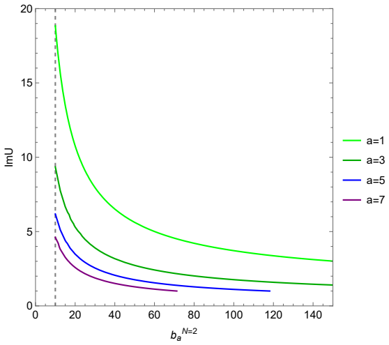
The load-bearing object is the perturbativity inequality (5.2), $16\pi^2 k_a \operatorname{Im} S > |\Delta_a|$, evaluated at $\mu^2 \sim M_{\text{string}}^2$, where $\Delta_a$ is the one-loop moduli-dependent threshold correction to the gauge coupling. The paper uses the classification of these threshold corrections by target-space duality symmetries, $PSL(2,\mathbb{Z})$, $\Gamma_0(n)$, and $\Gamma^0(n)$, together with explicit forms built from Dedekind eta functions such as $\operatorname{Im} T\,|\eta(T)|^4 \operatorname{Im} U\,|\eta(U)|^4$. In the region $\operatorname{Im} U > 1$, the eta function is approximated by $q^{1/24}$, which turns the inequality into an equation solved by the Lambert W function, yielding closed-form bounds on $\operatorname{Im} U$ and $\operatorname{Im} T$ as functions of $\operatorname{Im} S$, $b_a^{N=2}$, and the ratio $T/U$.
What would settle it
Compute the full one-loop threshold correction $\Delta_a$ from Eq. (3.3), including all twisted sectors and Green-Schwarz contributions, for a concrete $T^6/\mathbb{Z}_4$ or $T^6/\mathbb{Z}_{6-II}$ vacuum with $\operatorname{Im} S = 2$, $k_a = 1$, $|b_a^{N=2}| = 10$, $T = \omega$, and $\operatorname{Im} U = 40$. If the resulting corrected gauge coupling $16\pi^2 k_a \operatorname{Im} S - |\Delta_a|$ remains positive, then inequality (5.2) is not necessary and the bound $\operatorname{Im} U \lesssim 34.3$ is evaded.
Extended reading notes
Core claim
Within perturbative heterotic string theory on toroidal orbifolds, the paper's central claim is that perturbativity, meaning that the tree-level gauge coupling exceeds the one-loop moduli-dependent threshold correction, imposes necessary constraints on the modulus space of modular flavor models. Using threshold corrections classified by target-space duality symmetries $PSL(2,\mathbb{Z})$, $\Gamma_0(n)$, and $\Gamma^0(n)$, it derives bounds on $\operatorname{Im} U$ and $\operatorname{Im} T$ whose boundary is given by the Lambert W function. For representative values $\operatorname{Im} S \sim 2$, $k_a = 1$, and $|b_a^{N=2}| \sim 10$, fixing $T = \omega$ gives $\operatorname{Im} U \lesssim 34.3$; the constraints tighten as the dilaton decreases, the $\beta$-function coefficient increases, or the ratio $T/U$ grows. In the large-volume regime $T \gg 1$, almost all of the fundamental region is excluded and the allowed region concentrates near duality fixed points, with $\tau = i$ more strongly constrained than $\tau = \omega$; hence the paper concludes that $\tau \simeq i\infty$ lies in the Swampland and $\tau = i$ is disfavored.
Load-bearing premise
The whole derivation assumes that a heterotic vacuum is perturbatively valid exactly when the tree-level gauge coupling $16\pi^2 k_a \operatorname{Im} S$ exceeds the absolute value of the one-loop threshold correction $\Delta_a$, with $\Delta_a$ taken from the $N=2$ $\beta$-function sector only; if Green-Schwarz terms, other threshold sectors, or non-perturbative effects can cancel a large correction, the upper bounds do not follow.
Editorial extensions
If this is right
- The fixed point $\tau \simeq i\infty$, often used to generate hierarchical fermion masses, is not compatible with perturbative heterotic vacua at $\operatorname{Im} S \sim O(1)$ and $|b_a^{N=2}| \sim O(10)$.
- Radiative moduli stabilization scenarios that fix the modulus at $\operatorname{Im} \tau \sim O(10)$ are difficult to realize inside the perturbative regime.
- In the large-volume regime $T \gg 1$, almost all of the moduli space is excluded and the surviving region concentrates near an elliptic point of the duality group, with $\tau = \omega$ allowed and $\tau = i$ excluded for large enough volume.
- Increasing $|b_a^{N=2}|$ strengthens the bounds; for $b_a^{N=2} \gtrsim 90$ with $T = 7U$ and $\operatorname{Im} S = 2$, no point of the $PSL(2,\mathbb{Z})$ fundamental region remains perturbatively valid.
- The constraints depend on the ratio $T:U$; larger ratios of complex-structure to Kähler modulus give stronger bounds.
Reading between the lines
- Editorial inference: If the bounds hold, they give a top-down selection rule for modular flavor model building: among the fixed points $\tau = i\infty$, $i$, and $\omega$, only $\omega$ survives the large-volume limit, so models built near $\omega$ become the prime string-embedding candidates.
- Editorial inference: The same perturbativity argument could be turned into a scan over heterotic orbifold gauge groups, since for each model's $b_a^{N=2}$ and dilaton value the Lambert-W bound gives the full allowed region in $(T,U)$, which could be combined with moduli stabilization to test specific vacua.
- Editorial inference: A direct test would be to compute the exact one-loop threshold correction, not just the leading $N=2$ beta-function term, for a concrete orbifold near $\operatorname{Im} U \approx 34$; if the exact $\Delta_a$ stays below the tree-level coupling, the numerical cap is an artifact of the approximation.
Signed reviews
Editorial analysis
A structured set of objections, weighed in public.
Referee Report
Summary. This paper studies constraints on the moduli space of modular flavor models arising from one-loop moduli-dependent threshold corrections in perturbative heterotic string theory on toroidal orbifolds. After reviewing how modular flavor symmetries emerge from extra-dimensional wavefunctions, the authors import threshold formulas from Ref. [36] and group them into five classes according to target-space duality symmetries: PSL(2,Z) × PSL(2,Z), Γ0(2)-type groups, and Γ0(3)-type groups. The central step is inequality (5.2), which requires the tree-level dilaton contribution to the gauge coupling to dominate the one-loop threshold correction. Using the large-imaginary-part approximation for Dedekind eta functions, the authors derive analytic upper bounds on the imaginary parts of the complex-structure modulus U and the Kähler modulus T in terms of Lambert W functions, and they supplement these with numerical results in the region Im τ ≲ 1. The main quantitative claims are that for representative inputs (Im S = 2, k_a = 1, |b_a^{N=2}| = 10) the modulus is bounded by Im U ≲ 34.3 when T is fixed at the elliptic point ω, that larger ratios T/U and larger beta-function coefficients strengthen the bounds, and that in the large-volume regime the fixed point τ = i becomes disfavored while τ = ω remains allowed. The paper concludes with phenomenological implications for modular flavor model building and radiative moduli stabilization.
Significance. If the central inequality (5.2) were a necessary condition for perturbative heterotic vacua, the paper would provide a broadly useful top-down constraint on modular flavor model building, linking the modulus values used in bottom-up flavor fits to the validity of the string perturbation expansion. The paper has several genuine strengths: the Lambert W closed-form bounds are derived cleanly, the classification of threshold corrections into five duality-group classes is systematic, and the numerical analysis explicitly covers the region Im τ ≲ 1 where the analytic eta approximation fails. The authors are also transparent that the inputs Im S, k_a, and b_a^{N=2} are treated as scanned parameters rather than fitted to the output, so there is no disguised circularity. The main limitation is that the results are conditional on a specific model of the threshold corrections: the bounds are sufficient conditions for perturbativity under the retained N=2 threshold terms, not necessary string-theoretic constraints once Green-Schwarz constants and other one-loop sectors are included.
major comments (3)
- [Sec. 5, Eq. (5.2)] The inequality 16π² k_a Im S > |Δ_a| is presented as the condition ensuring weak gauge couplings at the string scale, and it is then used to derive upper bounds such as Eq. (5.10). However, this condition is sufficient rather than necessary: the full one-loop threshold correction contains moduli-independent and dilaton-dependent Green-Schwarz terms, and footnote 2 on page 7 explicitly drops the numerical constants associated with the Green-Schwarz function. Moreover, even within the retained N=2 pieces, other one-loop sectors or additional threshold contributions could partially cancel the moduli-dependent term. Consequently, the statement in the abstract that τ ≃ i∞ 'lies in the Swampland' is stronger than what the derivation supports. The paper should reframe Eq. (5.2) as a sufficient perturbativity constraint under the assumption that the exhibited N=2 threshold terms dominate, and either quantify the dropped Green-Schwarz constants or restrict the claims to cases where those constants are known to be negligible.
- [Sec. 4.3, Eqs. (4.12)-(4.13)] For groups (4) and (5), the coefficient Rhat b_a of the (I,θ³) sector is set equal to b_a^{N=2} 'for simplicity'. This is a choice, not a derivation: the orbifold relation (4.7) fixes b_a^{N=2} = 4 b^{(I,θ²)}_a but leaves Rhat b_a independent. Since the constraints (5.17)-(5.20) depend on Rhat b_a through terms with different moduli dependence (T, Rhat T, and the η(ω) contribution in Eq. (4.13)), the reported bounds for these groups are model-dependent. The authors should either derive Rhat b_a for the specific orbifolds listed in Sec. 4.3 or present the bounds as functions of the ratio Rhat b_a / b_a^{N=2} and explicitly state which ranges are covered by the figures.
- [Sec. 5.1, Eq. (5.10) and Figs. 2-5] The headline numerical result Im U ≲ 34.3 is obtained for the representative inputs Im S = 2, k_a = 1, and |b_a^{N=2}| = 10. These values are taken from MSSM gauge-coupling unification and typical beta-function magnitudes, but they are not derived for any concrete heterotic vacuum; in a given orbifold the beta-function coefficients, modular levels, and dilaton VEV are correlated, and the relevant threshold formula may not be the group (1) form. The paper should therefore label the quantitative bounds and the associated phenomenological conclusions in Sec. 6 as illustrative rather than as universal string-theoretic constraints, and it should indicate how the bounds change when the parameters are varied within ranges actually realized in the orbifold models of Sec. 4.3.
minor comments (6)
- [Footnote 2, p. 7] The name 'Green-Shwarz' is a typo; it should be 'Green-Schwarz'.
- [Sec. 3, Eqs. (3.6)-(3.7)] The same symbol Rbar Γ0(n) is defined in two different ways, once with c ≡ 0 mod n and once with b ≡ 0 mod n; the notation should distinguish Rbar Γ₀(n) from Rbar Γ⁰(n) or use different symbols to avoid confusion.
- [Sec. 4.1 and Sec. 4.3] The target-space duality group is written as Γ0_T(2) × (Γ_U)0(2) in Sec. 4.1 and as Γ0_T(2) × (Γ_U)0(2) in Eq. (4.10); please unify the notation for the upper and lower congruence subgroups.
- [Sec. 5.1, Eq. (5.4)] The sentence 'the RHS can be calculated as follows' presents the numerical value 0.680... without specifying the minimizing point of T₂|η(T)|⁴ U₂|η(U)|⁴; adding that the minimum occurs at T = U = ω would make the derivation easier to follow.
- [Sec. 5.2, captions of Figs. 10 and 13] The captions 'These are the boundaries concerning 7T = U' and 'concerning 7T = U, Rhat T = T, Rhat U = T' are terse; please state explicitly that Im S = 2 is fixed and indicate which axis corresponds to the plotted modulus.
- [Sec. 6, Fig. 16] The claim that 'the larger the volume of extra dimensional space, the stronger the stringy constraints' is inferred from a few values T = 10i, 10.02i, 10.04i, 10.06i; please clarify whether this is a numerical trend observed in the plotted examples or an analytic property of Eq. (5.3).
Circularity Check
No significant circularity: the modulus bounds are derived from external threshold formulas plus a stated perturbativity assumption, with all inputs scanned rather than fitted.
full rationale
The central derivation is self-contained against external benchmarks. The load-bearing inequality Eq. (5.2), 16 pi^2 k_a ImS > |Delta_a|, is introduced as an explicit assumption rather than as a fitted or predicted quantity; the paper states that it assumes gauge couplings are weak enough at the string scale, then derives the inequality from Eq. (3.2). The threshold corrections Delta_a are taken from external Refs. [33,34,36], and the five groups in Sec. 4.3 classify those existing formulas rather than introducing a new ansatz. The numerical inputs ImS ~ 2, k_a = 1, and |b_a^{N=2}| ~ O(10) are stated as typical or scanned values, and the figures vary them systematically; no parameter is fitted to the target bound and then renamed a prediction. The Lambert-W bounds in Eqs. (5.10)-(5.20) are algebraic rearrangements of the inequality, so they inherit the stated perturbativity assumption but do not reduce to the inputs by construction. The self-citations to Refs. [30,31,32] appear in the motivational discussion of flux landscapes, and the claimed exclusion of tau ~ i infinity and the large-volume disfavoring of tau = i do not rely on those citations. Two acknowledged modeling choices (footnote 2 dropping Green-Schwarz numerical constants; Sec. 4.3 setting the hatted coefficient equal to b_a^{N=2} for simplicity) weaken the string-theoretic necessity of the bounds but are stated assumptions, not disguised inputs. Hence the central claim has independent content and no circular step reduces to its own inputs by definition.
Assumptions & free parameters
free parameters (5)
- beta-function coefficient |b^{N=2}_a| =
10 as typical, scanned up to 140
- dilaton ImS =
2 as benchmark, scanned 0.5 to 4
- Kac-Moody level k_a =
1
- ratio a in T = aU =
scanned from 1 to 7
- ratios b and c in group (4) =
scanned from 1 to 3
assumptions (5)
- domain assumption Threshold correction formula Eq. (3.3) and the classified forms Eqs. (4.9) to (4.13) from Refs. [33,34,36] are correct for these orbifolds.
- domain assumption Perturbativity demands 16 pi^2 k_a ImS > |Delta_a| at mu^2 ~ M_string^2, Eq. (5.2).
- ad hoc to paper Green-Schwarz numerical constants can be neglected; only beta-function coefficients matter in Delta_a.
- ad hoc to paper For groups (4) and (5), the hatted beta coefficient is set equal to b^{N=2}_a.
- domain assumption Dedekind eta q-series approximation Im tau |eta(tau)|^4 approximately Im tau exp(-pi Im tau / 3) for Im tau > 1, Eq. (5.7).
Cite this review
Pith. "Pith review of Stringy Constraints on Modular Flavor Models." pith.science (2026). https://pith.science/paper/F2WPYSCQ
@misc{pith2026250812392,
  author       = {Pith},
  title        = {Pith review of: Stringy Constraints on Modular Flavor Models},
  year         = {2026},
  howpublished = {\url{https://pith.science/paper/F2WPYSCQ}},
  note         = {Machine review of arXiv:2508.12392}
}
abstract
We investigate stringy constraints on moduli spaces in modular flavor models by analyzing moduli-dependent threshold corrections in heterotic string vacua. While moduli play a crucial role in determining the flavor structure of fermions predicted by modular flavor models, the parameter space in which their vacuum expectation values are allowed has not been fully explored. In this work, within the framework of perturbative heterotic string theory on toroidal orbifolds, we derive constraints on the moduli space and study their systematic behavior. We characterize the stringy constraints in terms of the dilaton, the beta-function coefficients, and the ratio between a complex-structure modulus and a K\"ahler modulus. It is found that the large value of the modulus controlling the flavor structure, i.e., $\tau\simeq i \infty$, lies in the Swampland, and the self-dual point $\tau=i$ is also disfavored in the large volume regime of toroidal backgrounds. In addition, we discuss the phenomenological implications of these stringy constraints.
Figures


Figures from the paper (14 more)



Forward citations
Cited by 1 Pith paper
-
Fibre Inflation Meets Quintessence: Implications of Perturbative Stabilisation
Adding a base-modulus redefinition to fibre inflation in perturbative LVS shifts (ns, r) into ACT-allowed territory and yields an axion quintessence companion.
Reference graph
Works this paper leans on
- [36]
-
[1]
Altarelli and F
G. Altarelli and F. Feruglio,Discrete flavor symmetries and models of neutrino mixing, Reviews of Modern Physics82 (2010) 2701–2729
2010
-
[2]
Ishimori, T
H. Ishimori, T. Kobayashi, H. Ohki, Y. Shimizu, H. Okada and M. Tanimoto,Non-abelian discrete symmetries in particle physics, Progress of Theoretical Physics Supplement183 (2010) 1–163
2010
-
[3]
King and C
S.F. King and C. Luhn,Neutrino mass and mixing with discrete symmetry, Reports on Progress in Physics76 (2013) 056201
2013
-
[4]
King,Models of neutrino mass, mixing and cp violation, 2015
S.F. King,Models of neutrino mass, mixing and cp violation, 2015
2015
-
[5]
T. Kobayashi, H. Ohki, H. Okada, Y. Shimizu and M. Tanimoto,An Introduction to Non-Abelian Discrete Symmetries for Particle Physicists(1, 2022), 10.1007/978-3-662-64679-3
-
[6]
R. de Adelhart Toorop, F. Feruglio and C. Hagedorn,Finite Modular Groups and Lepton Mixing, Nucl. Phys. B 858 (2012) 437 [1112.1340]
arXiv 2012
-
[7]
F. Feruglio,Are neutrino masses modular forms?, inFrom My Vast Repertoire ...: Guido Altarelli’s Legacy, A. Levy, S. Forte and G. Ridolfi, eds., pp. 227–266 (2019), DOI [1706.08749]
arXiv 2019
Show all 88 references
-
[8]
Kobayashi and M
T. Kobayashi and M. Tanimoto,Modular flavor symmetric models, 7, 2023 [2307.03384]
2023 arXiv
-
[9]
Ding and S.F
G.-J. Ding and S.F. King,Neutrino Mass and Mixing with Modular Symmetry, 2311.09282
-
[10]
Kobayashi, K
T. Kobayashi, K. Tanaka and T.H. Tatsuishi,Neutrino mixing from finite modular groups, Phys. Rev. D98 (2018) 016004 [1803.10391]
2018 arXiv
-
[11]
Penedo and S.T
J.T. Penedo and S.T. Petcov,Lepton Masses and Mixing from ModularS4 Symmetry, Nucl. Phys. B 939 (2019) 292 [1806.11040]. – 29 –
2019 arXiv
-
[12]
Novichkov, J.T
P.P. Novichkov, J.T. Penedo, S.T. Petcov and A.V. Titov,Modular A5 symmetry for flavour model building, JHEP 04 (2019) 174 [1812.02158]
2019 arXiv
-
[13]
Strominger and E
A. Strominger and E. Witten,New Manifolds for Superstring Compactification, Commun. Math. Phys. 101 (1985) 341
1985
-
[14]
Candelas,Yukawa couplings between (2, 1)-forms, Nuclear Physics B298 (1988) 458
P. Candelas,Yukawa couplings between (2, 1)-forms, Nuclear Physics B298 (1988) 458
1988
-
[15]
Dixon, V.S
L.J. Dixon, V.S. Kaplunovsky and J. Louis,On effective field theories describing (2, 2) vacua of the heterotic string, Nuclear Physics B329 (1990) 27
1990
-
[16]
Cremades, L.E
D. Cremades, L.E. Ibanez and F. Marchesano,Computing Yukawa couplings from magnetized extra dimensions, JHEP 05 (2004) 079 [hep-th/0404229]
2004 arXiv
-
[17]
Ferrara, D
S. Ferrara, D. Lüst and S. Theisen,Target space modular invariance and low-energy couplings in orbifold compacifications, Physics Letters B233 (1989) 147
1989
-
[18]
Ferrara, .D
S. Ferrara, .D. Lust and S. Theisen,Target Space Modular Invariance and Low-Energy Couplings in Orbifold Compactifications, Phys. Lett. B233 (1989) 147
1989
-
[19]
Lerche, D
W. Lerche, D. Lust and N.P. Warner,Duality Symmetries inN = 2 Landau-ginzburg Models, Phys. Lett. B231 (1989) 417
1989
-
[20]
Lauer, J
J. Lauer, J. Mas and H.P. Nilles,Twisted sector representations of discrete background symmetries for two-dimensional orbifolds, Nucl. Phys. B 351 (1991) 353
1991
-
[21]
Nilles, S
H.P. Nilles, S. Ramos-Sanchez, A. Trautner and P.K.S. Vaudrevange,Orbifolds from Sp(4,Z) and their modular symmetries, Nucl. Phys. B 971 (2021) 115534 [2105.08078]
2021 arXiv
-
[22]
Kobayashi and S
T. Kobayashi and S. Nagamoto,Zero-modes on orbifolds: Magnetized orbifold models by modular transformation, Physical Review D96 (2017)
2017
-
[23]
Kobayashi, S
T. Kobayashi, S. Nagamoto, S. Takada, S. Tamba and T.H. Tatsuishi,Modular symmetry and non-Abelian discrete flavor symmetries in string compactification, Phys. Rev. D97 (2018) 116002 [1804.06644]
2018 arXiv
-
[24]
Kobayashi and S
T. Kobayashi and S. Tamba,Modular forms of finite modular subgroups from magnetized D-brane models, Phys. Rev. D99 (2019) 046001 [1811.11384]
2019 arXiv
-
[25]
H. Ohki, S. Uemura and R. Watanabe,Modular flavor symmetry on a magnetized torus, Phys. Rev. D102 (2020) 085008 [2003.04174]
2020 arXiv
-
[26]
Kikuchi, T
S. Kikuchi, T. Kobayashi, S. Takada, T.H. Tatsuishi and H. Uchida,Revisiting modular symmetry in magnetized torus and orbifold compactifications, Phys. Rev. D102 (2020) 105010 [2005.12642]
2020 arXiv
-
[27]
Kikuchi, T
S. Kikuchi, T. Kobayashi, H. Otsuka, S. Takada and H. Uchida,Modular symmetry by orbifolding magnetizedT 2×T 2: realization of double cover ofΓN, JHEP 11 (2020) 101 [2007.06188]
2020 arXiv
-
[28]
Kikuchi, T
S. Kikuchi, T. Kobayashi and H. Uchida,Modular flavor symmetries of three-generation modes on magnetized toroidal orbifolds, Phys. Rev. D104 (2021) 065008 [2101.00826]
2021 arXiv
-
[29]
Almumin, M.-C
Y. Almumin, M.-C. Chen, V. Knapp-Pérez, S. Ramos-Sánchez, M. Ratz and S. Shukla, Metaplectic Flavor Symmetries from Magnetized Tori, JHEP 05 (2021) 078 [2102.11286]
2021 arXiv
-
[30]
Ishiguro, T
K. Ishiguro, T. Kobayashi and H. Otsuka,Landscape of Modular Symmetric Flavor Models, JHEP 03 (2021) 161 [2011.09154]. – 30 –
2021 arXiv
-
[31]
Ishiguro, T
K. Ishiguro, T. Kai, T. Kobayashi and H. Otsuka,Flux Landscape with enhanced symmetry not on SL(2,Z) elliptic points, JHEP 02 (2024) 099 [2311.12425]
2024 arXiv
-
[32]
Ishiguro, T
K. Ishiguro, T. Kai, T. Kobayashi, Y. Koga and H. Otsuka,Classification of Modular Symmetries in Type IIB Flux Landscape, 2502.20743
-
[33]
Kaplunovsky,One-loop threshold effects in string unification, 1992
V. Kaplunovsky,One-loop threshold effects in string unification, 1992
1992
-
[34]
Dixon, V
L.J. Dixon, V. Kaplunovsky and J. Louis,Moduli dependence of string loop corrections to gauge coupling constants, Nucl. Phys. B 355 (1991) 649
1991
-
[35]
Kaplunovsky and J
V. Kaplunovsky and J. Louis,On gauge couplings in string theory, Nuclear Physics B444 (1995) 191–244
1995
-
[37]
Kikuchi, T
S. Kikuchi, T. Kobayashi, H. Otsuka, M. Tanimoto, H. Uchida and K. Yamamoto,4D modular flavor symmetric models inspired by a higher-dimensional theory, Phys. Rev. D106 (2022) 035001 [2201.04505]
2022 arXiv
-
[38]
Ishiguro, T
K. Ishiguro, T. Kobayashi and H. Otsuka,Spontaneous CP violation and symplectic modular symmetry in Calabi-Yau compactifications, Nucl. Phys. B 973 (2021) 115598 [2010.10782]
2021 arXiv
-
[39]
Ishiguro, T
K. Ishiguro, T. Kobayashi and H. Otsuka,Symplectic modular symmetry in heterotic string vacua: flavor, CP, and R-symmetries, JHEP 01 (2022) 020 [2107.00487]
2022 arXiv
-
[40]
Ishiguro, T
K. Ishiguro, T. Kobayashi, S. Nishimura and H. Otsuka,Modular forms and hierarchical Yukawa couplings in heterotic Calabi-Yau compactifications, JHEP 08 (2024) 088 [2402.13563]
2024 arXiv
-
[41]
Abe, K.-S
H. Abe, K.-S. Choi, T. Kobayashi and H. Ohki,Higher Order Couplings in Magnetized Brane Models, JHEP 06 (2009) 080 [0903.3800]
2009 arXiv
-
[42]
Honda, T
M. Honda, T. Kobayashi and H. Otsuka,Zero-mode product expansions and higher order couplings in gauge backgrounds, Phys. Rev. D100 (2019) 025015 [1812.03357]
2019 arXiv
-
[43]
Ishiguro, H
K. Ishiguro, H. Okada and H. Otsuka,Residual flavor symmetry breaking in the landscape of modular flavor models, JHEP 09 (2022) 072 [2206.04313]
2022 arXiv
-
[44]
Novichkov, J.T
P.P. Novichkov, J.T. Penedo and S.T. Petcov,Modular flavour symmetries and modulus stabilisation, JHEP 03 (2022) 149 [2201.02020]
2022 arXiv
-
[45]
Knapp-Perez, X.-G
V. Knapp-Perez, X.-G. Liu, H.P. Nilles, S. Ramos-Sanchez and M. Ratz,Matter matters in moduli fixing and modular flavor symmetries, Phys. Lett. B844 (2023) 138106 [2304.14437]
2023 arXiv
-
[46]
Kobayashi, K
T. Kobayashi, K. Nasu, R. Sakuma and Y. Yamada,Radiative correction on moduli stabilization in modular flavor symmetric models, Phys. Rev. D108 (2023) 115038 [2310.15604]
2023 arXiv
-
[47]
Higaki, J
T. Higaki, J. Kawamura and T. Kobayashi,Finite modular axion and radiative moduli stabilization, JHEP 04 (2024) 147 [2402.02071]
2024 arXiv
-
[48]
Kobayashi and H
T. Kobayashi and H. Otsuka,Challenge for spontaneousCP violation in Type IIB orientifolds with fluxes, Phys. Rev. D102 (2020) 026004 [2004.04518]
2020 arXiv
-
[49]
Higaki, T
T. Higaki, T. Kobayashi, K. Nasu and H. Otsuka,Spontaneous CP violation and partially broken modular flavor symmetries, JHEP 09 (2024) 024 [2405.18813]. – 31 –
2024 arXiv
-
[50]
Novichkov, J.T
P.P. Novichkov, J.T. Penedo, S.T. Petcov and A.V. Titov,Modular S4 models of lepton masses and mixing, JHEP 04 (2019) 005 [1811.04933]
2019 arXiv
-
[51]
Novichkov, S.T
P.P. Novichkov, S.T. Petcov and M. Tanimoto,Trimaximal Neutrino Mixing from Modular A4 Invariance with Residual Symmetries, Phys. Lett. B793 (2019) 247 [1812.11289]
2019 arXiv
-
[52]
Ding, S.F
G.-J. Ding, S.F. King, X.-G. Liu and J.-N. Lu,Modular S4 and A4 symmetries and their fixed points: new predictive examples of lepton mixing, JHEP 12 (2019) 030 [1910.03460]
2019
-
[53]
Okada and M
H. Okada and M. Tanimoto,Towards unification of quark and lepton flavors inA4 modular invariance, Eur. Phys. J. C81 (2021) 52 [1905.13421]
2021 arXiv
-
[54]
King and Y.-L
S.F. King and Y.-L. Zhou,Trimaximal TM1 mixing with two modularS4 groups, Phys. Rev. D 101 (2020) 015001 [1908.02770]
2020 arXiv
-
[55]
Okada and M
H. Okada and M. Tanimoto,Quark and lepton flavors with common modulusτ in A4 modular symmetry, Phys. Dark Univ.40 (2023) 101204 [2005.00775]
2023 arXiv
-
[56]
Okada and M
H. Okada and M. Tanimoto,Modular invariant flavor model ofA4 and hierarchical structures at nearby fixed points, Phys. Rev. D103 (2021) 015005 [2009.14242]
2021 arXiv
-
[57]
Okada and M
H. Okada and M. Tanimoto,Spontaneous CP violation by modulusτ in A4 model of lepton flavors, JHEP 03 (2021) 010 [2012.01688]
2021 arXiv
-
[58]
Feruglio, V
F. Feruglio, V. Gherardi, A. Romanino and A. Titov,Modular invariant dynamics and fermion mass hierarchies aroundτ =i, JHEP 05 (2021) 242 [2101.08718]
2021 arXiv
-
[59]
Kobayashi, H
T. Kobayashi, H. Otsuka, M. Tanimoto and K. Yamamoto,Modular symmetry in the SMEFT, Phys. Rev. D105 (2022) 055022 [2112.00493]
2022 arXiv
-
[60]
Kobayashi, H
T. Kobayashi, H. Otsuka, M. Tanimoto and K. Yamamoto,Lepton flavor violation, lepton (g − 2)µ,e and electron EDM in the modular symmetry, JHEP 08 (2022) 013 [2204.12325]
2022 arXiv
-
[61]
Kobayashi, H
T. Kobayashi, H. Okada and Y. Orikasa,Dark matter stability at fixed points in a modular A4 symmetry, Phys. Dark Univ.37 (2022) 101080 [2111.05674]
2022 arXiv
-
[62]
Mayr and S
P. Mayr and S. Stieberger,Threshold corrections to gauge couplings in orbifold compactifications, Nucl. Phys. B 407 (1993) 725 [hep-th/9303017]
1993 arXiv
-
[63]
Erler and A
J. Erler and A. Klemm,Comment on the generation number in orbifold compactifications, Communications in Mathematical Physics153 (1993) 579–604
1993
-
[64]
Witten,Dimensional reduction of superstring models, Physics Letters B155 (1985) 151
E. Witten,Dimensional reduction of superstring models, Physics Letters B155 (1985) 151
1985
-
[65]
Kaplunovsky and J
V. Kaplunovsky and J. Louis,Field dependent gauge couplings in locally supersymmetric effective quantum field theories, Nuclear Physics B422 (1994) 57–124
1994
-
[66]
Mayr and S
P. Mayr and S. Stieberger,Dilaton, antisymmetric tensor and gauge fields in string effective theories at the one-loop level, Nuclear Physics B412 (1994) 502–522
1994
-
[67]
Kikuchi, T
S. Kikuchi, T. Kobayashi, K. Nasu, S. Takada and H. Uchida,Quark mass hierarchies and CP violation in A4 × A4 × A4 modular symmetric flavor models, JHEP 07 (2023) 134 [2302.03326]
2023 arXiv
-
[68]
Petcov and M
S.T. Petcov and M. Tanimoto,A4 modular flavour model of quark mass hierarchies close to the fixed pointτ = i∞, JHEP 08 (2023) 086 [2306.05730]
2023 arXiv
-
[69]
Y. Abe, T. Higaki, J. Kawamura and T. Kobayashi,Quark masses and CKM hierarchies fromS′ 4 modular flavor symmetry, Eur. Phys. J. C83 (2023) 1140 [2301.07439]. – 32 –
2023 arXiv
-
[70]
Y. Abe, T. Higaki, J. Kawamura and T. Kobayashi,Quark and lepton hierarchies from S4’ modular flavor symmetry, Phys. Lett. B842 (2023) 137977 [2302.11183]
2023 arXiv
-
[71]
Kikuchi, T
S. Kikuchi, T. Kobayashi, K. Nasu, S. Takada and H. Uchida,Quark hierarchical structures in modular symmetric flavor models at level 6, Phys. Rev. D107 (2023) 055014 [2301.03737]
2023 arXiv
-
[72]
Y. Abe, T. Higaki, J. Kawamura and T. Kobayashi,Fermion hierarchies inSU (5) grand unification fromΓ′ 6 modular flavor symmetry, JHEP 08 (2023) 097 [2307.01419]
2023 arXiv
-
[73]
Hai, A.R
M. Hai, A.R. Kamal, N.F. Shamma and M.S.J. Shuvo,Perturbative Kähler Moduli Inflation, 2506.08083
-
[74]
Feruglio,Universal Predictions of Modular Invariant Flavor Models near the Self-Dual Point, Phys
F. Feruglio,Universal Predictions of Modular Invariant Flavor Models near the Self-Dual Point, Phys. Rev. Lett.130 (2023) 101801 [2211.00659]
2023 arXiv
-
[75]
Feruglio, V
F. Feruglio, V. Gherardi, A. Romanino and A. Titov,Modular invariant dynamics and fermion mass hierarchies aroundτ =i, Journal of High Energy Physics2021 (2021)
2021
-
[76]
Novichkov, J.T
P.P. Novichkov, J.T. Penedo and S.T. Petcov,Fermion mass hierarchies, large lepton mixing and residual modular symmetries, JHEP 04 (2021) 206 [2102.07488]
2021 arXiv
-
[77]
Petcov and M
S.T. Petcov and M. Tanimoto,A4 modular flavour model of quark mass hierarchies close to the fixed pointτ =ω, Eur. Phys. J. C83 (2023) 579 [2212.13336]
2023 arXiv
-
[78]
de Medeiros Varzielas, M
I. de Medeiros Varzielas, M. Levy, J.T. Penedo and S.T. Petcov,Quarks at the modular S4 cusp, JHEP 09 (2023) 196 [2307.14410]
2023 arXiv
-
[79]
H. Abe, T. Kobayashi and H. Otsuka,Natural inflation with and without modulations in type IIB string theory, JHEP 04 (2015) 160 [1411.4768]
2015 arXiv
-
[80]
Ding, S.-Y
G.-J. Ding, S.-Y. Jiang and W. Zhao,Modular invariant slow roll inflation, JCAP 10 (2024) 016 [2405.06497]
2024 arXiv
-
[81]
Baur, H.P
A. Baur, H.P. Nilles, A. Trautner and P.K.S. Vaudrevange,Unification of Flavor, CP, and Modular Symmetries, Phys. Lett. B795 (2019) 7 [1901.03251]
2019 arXiv
-
[82]
Baur, H.P
A. Baur, H.P. Nilles, A. Trautner and P.K.S. Vaudrevange,A String Theory of Flavor and C P, Nucl. Phys. B 947 (2019) 114737 [1908.00805]
2019 arXiv
-
[83]
Nilles, S
H.P. Nilles, S. Ramos-Sánchez and P.K.S. Vaudrevange,Eclectic Flavor Groups, JHEP 02 (2020) 045 [2001.01736]
2020 arXiv
-
[84]
Nilles, S
H.P. Nilles, S. Ramos-Sanchez and P.K.S. Vaudrevange,Lessons from eclectic flavor symmetries, Nucl. Phys. B 957 (2020) 115098 [2004.05200]
2020 arXiv
-
[85]
Nilles, S
H.P. Nilles, S. Ramos–Sánchez and P.K.S. Vaudrevange,Eclectic flavor scheme from ten-dimensional string theory – I. Basic results, Phys. Lett. B808 (2020) 135615 [2006.03059]
2020 arXiv
-
[86]
A. Baur, M. Kade, H.P. Nilles, S. Ramos-Sanchez and P.K.S. Vaudrevange,The eclectic flavor symmetry of theZ2 orbifold, JHEP 02 (2021) 018 [2008.07534]
2021 arXiv
-
[87]
Nilles, S
H.P. Nilles, S. Ramos–Sánchez and P.K.S. Vaudrevange,Eclectic flavor scheme from ten-dimensional string theory - II detailed technical analysis, Nucl. Phys. B 966 (2021) 115367 [2010.13798]
2021 arXiv
-
[88]
Ishiguro, T
K. Ishiguro, T. Kobayashi and H. Otsuka,Hierarchical structure of physical Yukawa couplings from matter field Kähler metric, JHEP 07 (2021) 064 [2103.10240]. – 33 –
2021 arXiv
Reviewed August 15, 2026 · model on record in the stance chip above.
Discussion (0). Continue with ORCID to comment.