EAGT: Echocardiography Augmentation for Generalisability and Transferability
Pith reviewed 2026-05-20 20:36 UTC · model grok-4.3
The pith
Anatomically plausible geometric augmentations improve cross-dataset performance in echocardiography segmentation models.
A machine-rendered reading of the paper's core claim, the machinery that carries it, and where it could break.
Core claim
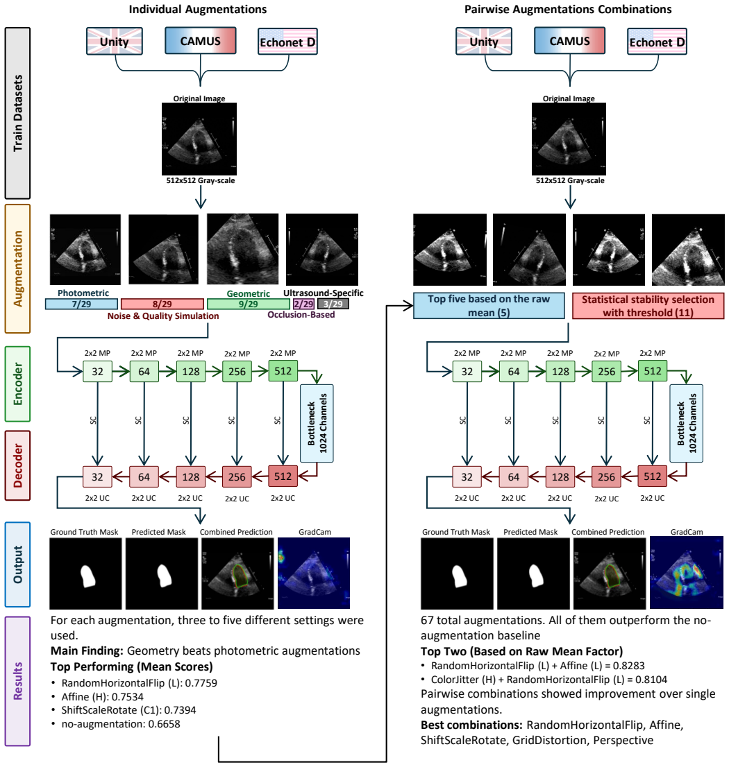
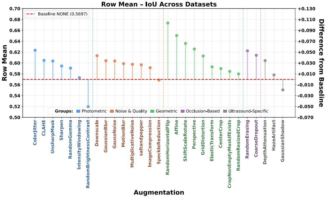
The paper establishes through extensive experiments that geometric data augmentations preserving anatomical structure lead to better generalisability and transferability of echocardiography segmentation models across institutions and scanners, with specific pairwise combinations providing superior results compared to individual or intensity-based methods.
What carries the argument
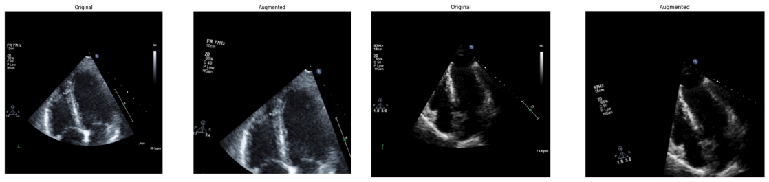
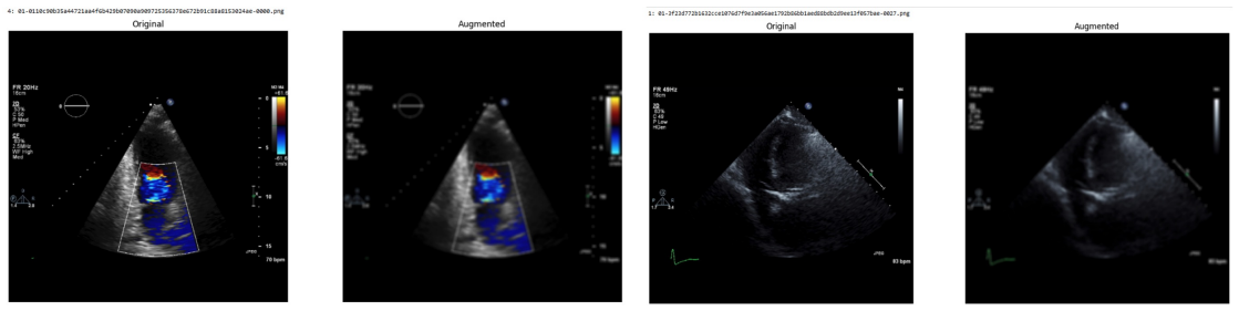
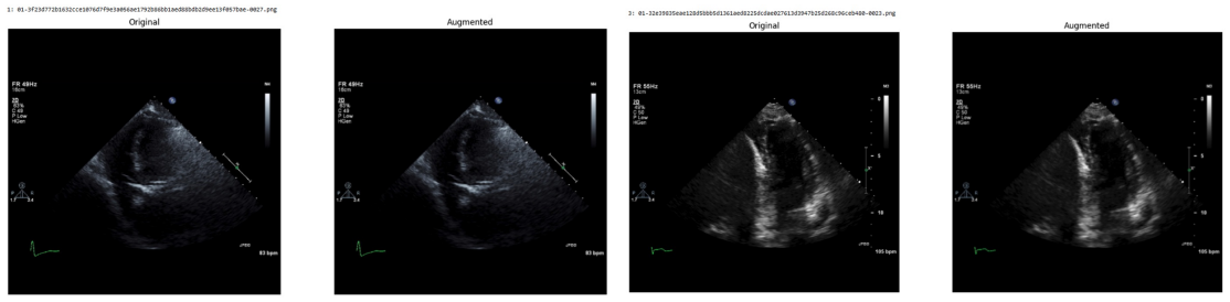
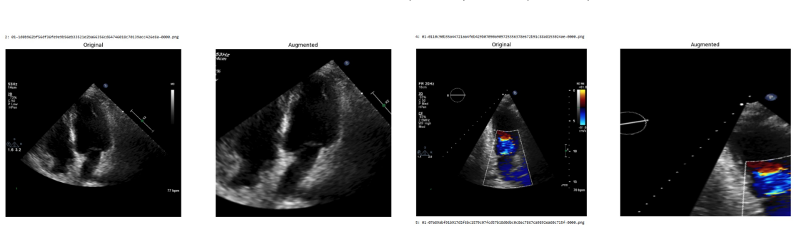
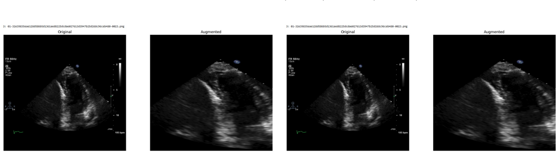
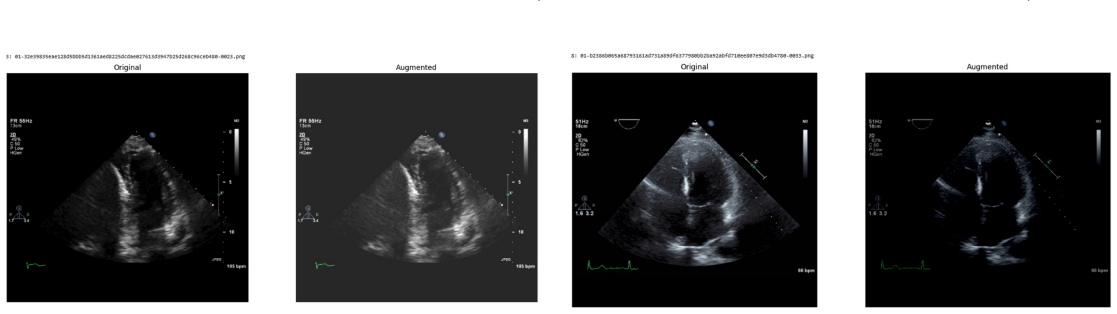
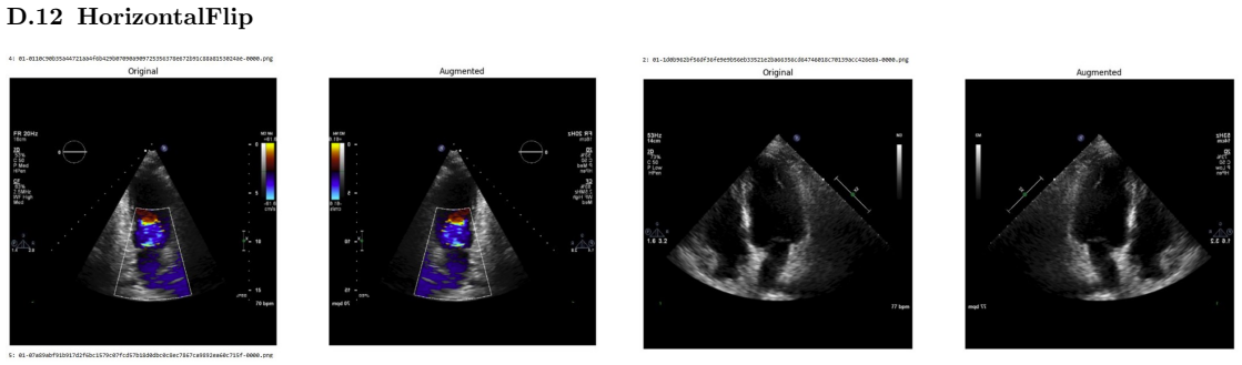
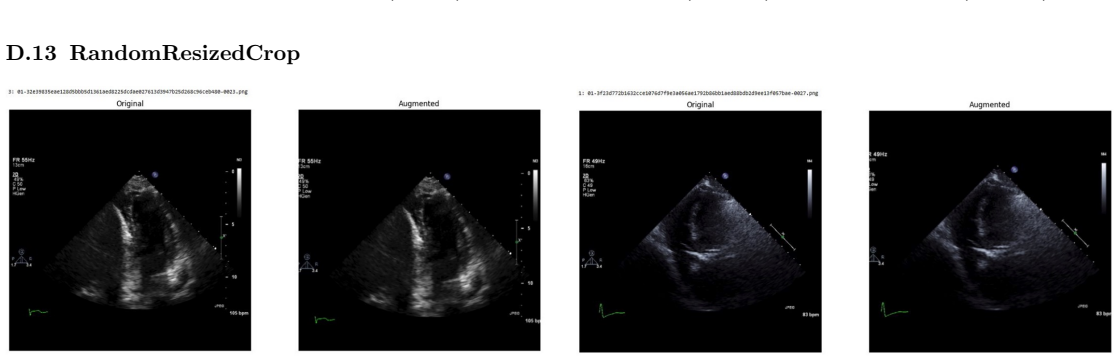
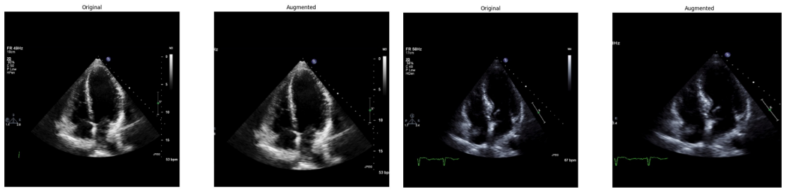
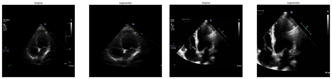
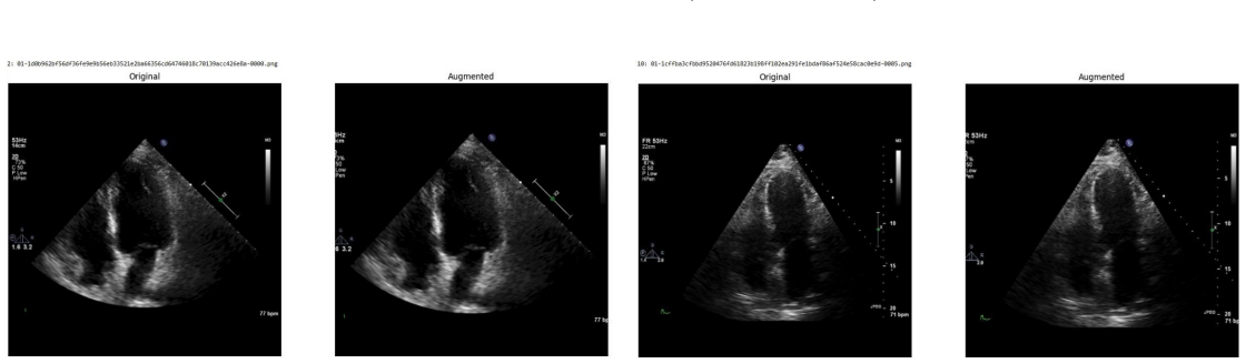
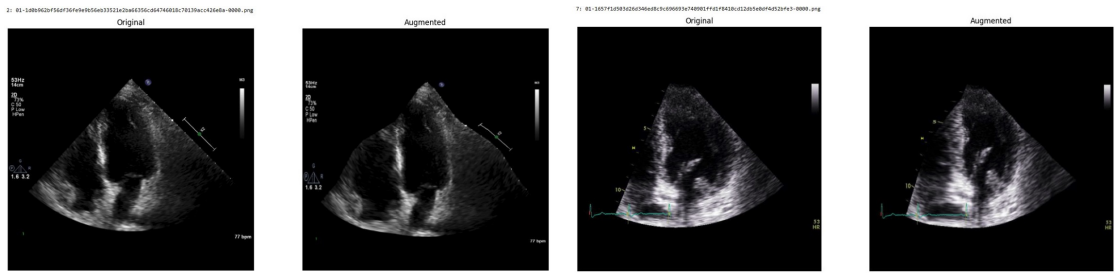
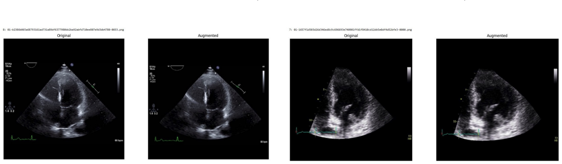
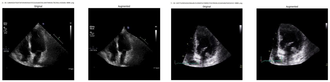
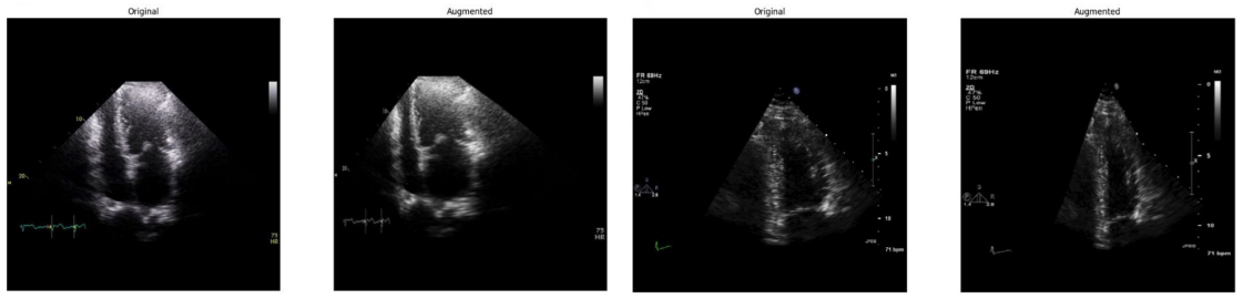
Systematic testing of geometric transformations such as affine and random horizontal flip, applied during training of U-Net models for 2D left ventricular segmentation, to enhance model robustness to dataset shifts.
If this is right
- Geometric augmentations lead to higher Dice and IoU scores in cross-dataset evaluation scenarios.
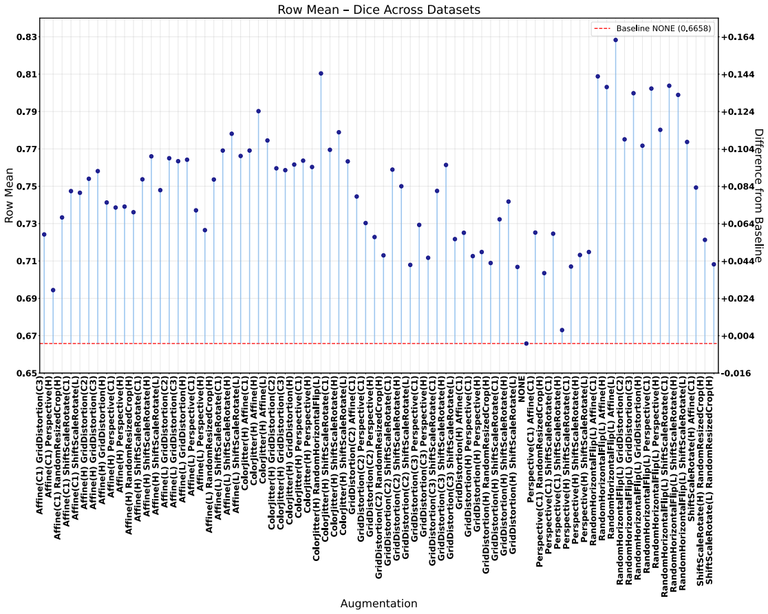
- Combinations of augmentations, particularly flip with affine, outperform single augmentations in transfer tasks.
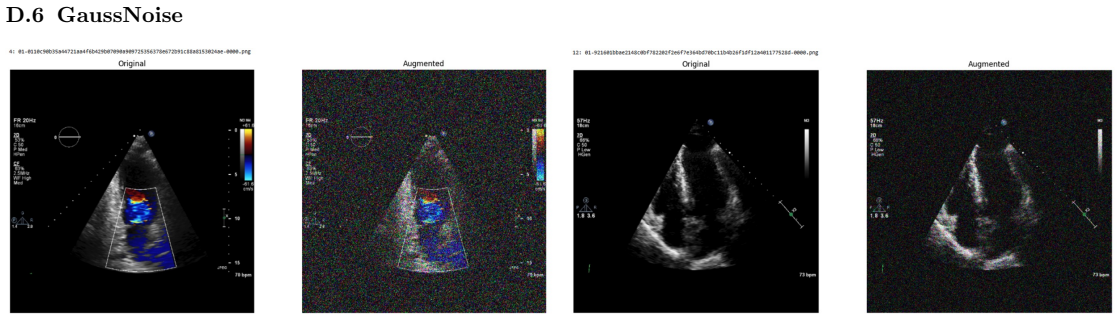
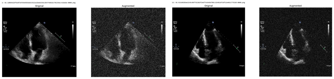
- Avoiding aggressive intensity augmentations prevents degradation of model generalisability.
- These augmentation strategies provide empirically supported guidance for improving model transferability in echocardiography analysis.
Where Pith is reading between the lines
- If validated further, these augmentation choices could reduce the need for extensive new data collection in clinical AI deployment.
- Similar principles might apply to segmentation tasks in other ultrasound or imaging modalities facing domain shifts.
- Exploring these augmentations on models beyond U-Net could test the broader applicability of the findings.
- Integrating these policies into standard training pipelines may improve real-world performance of automated cardiac analysis tools.
Load-bearing premise
The variability across the three chosen datasets sufficiently represents differences in scanners, institutions, and patient populations encountered in practice.
What would settle it
Evaluating the top-performing augmentation combinations on an additional echocardiography dataset from a new source and finding no statistically significant improvement in cross-dataset metrics would falsify the central claim.
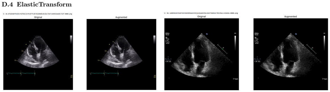
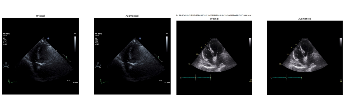
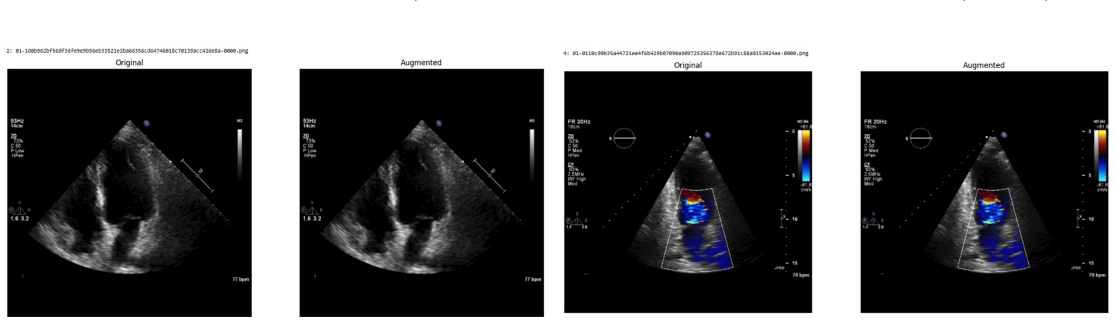
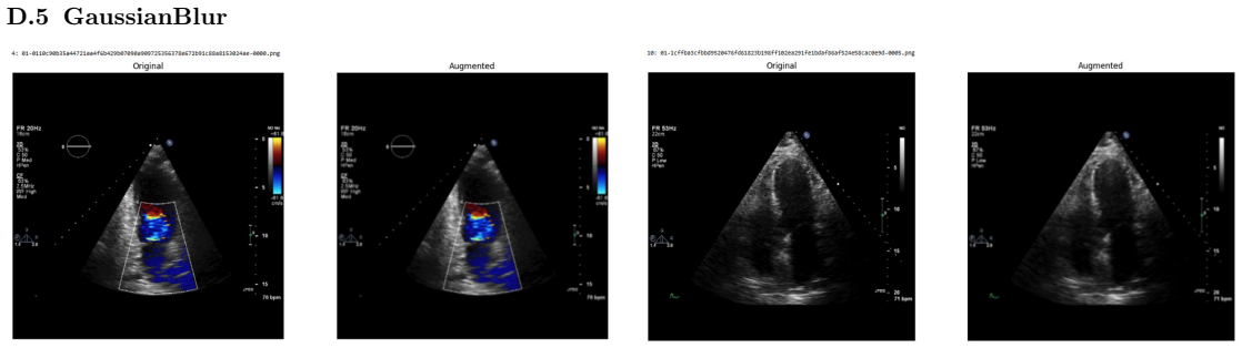
Figures


read the original abstract
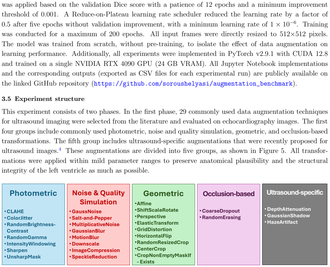
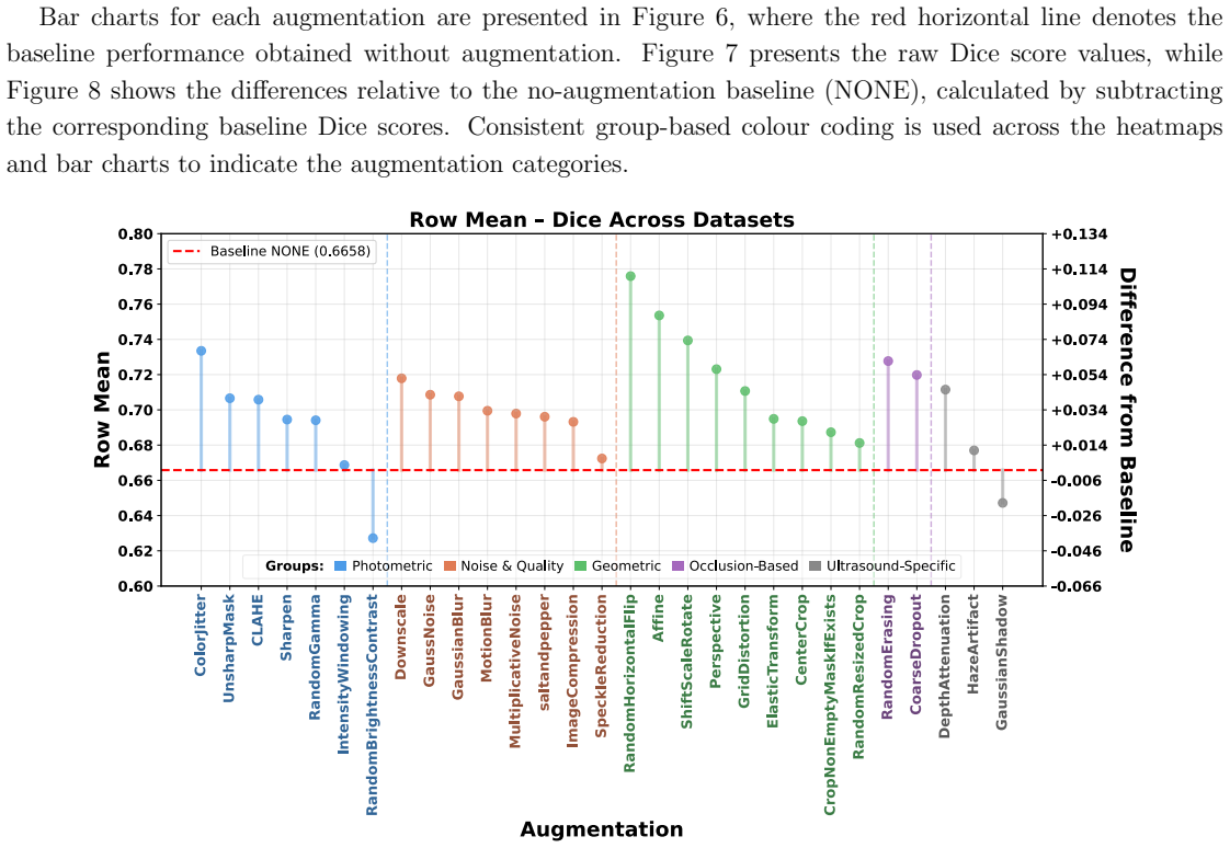
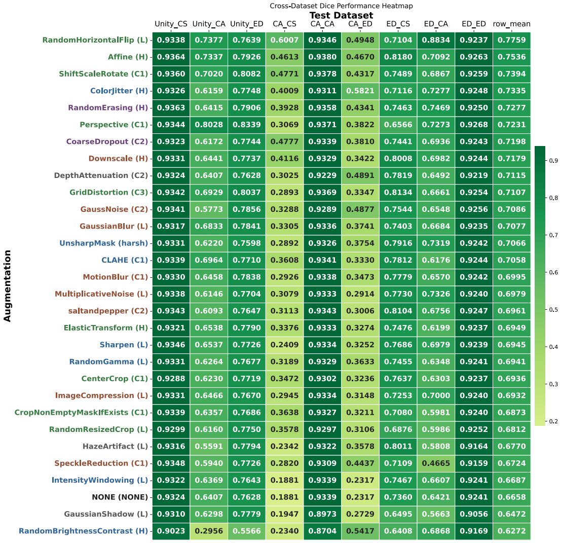
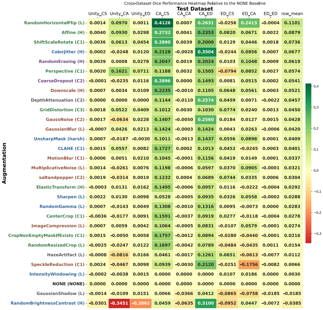
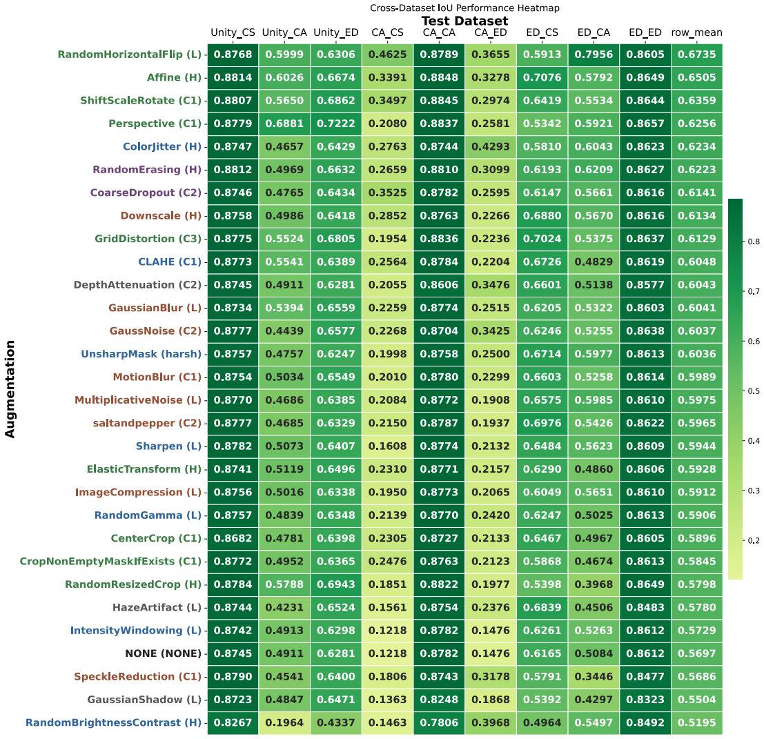
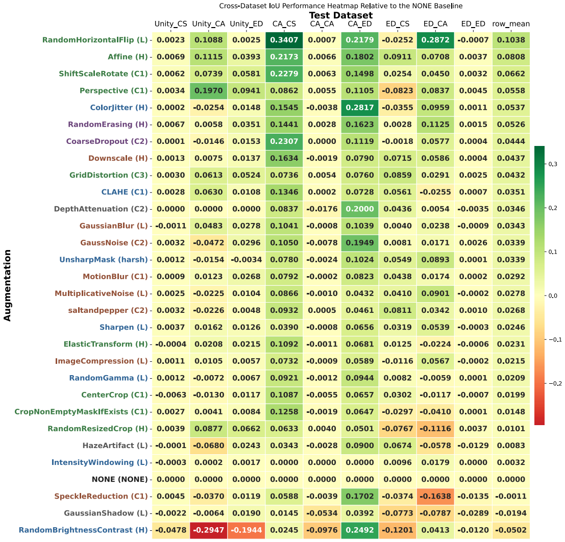
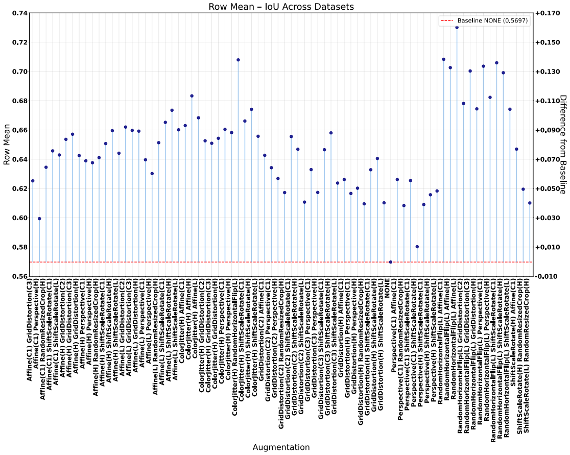
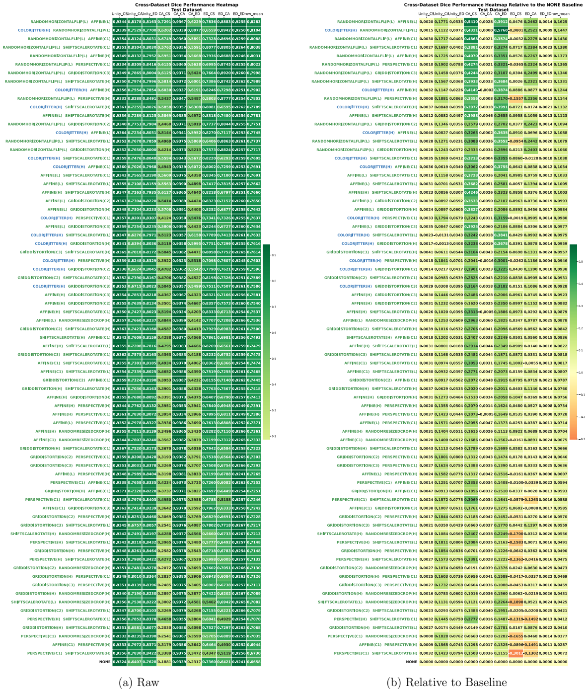
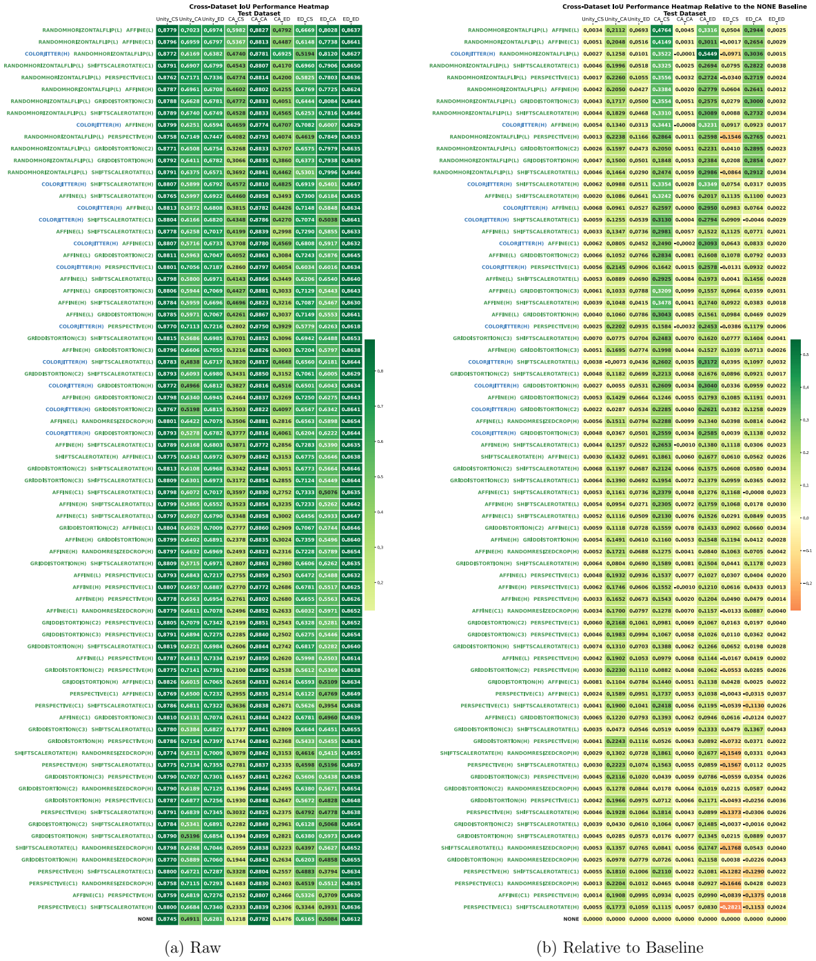
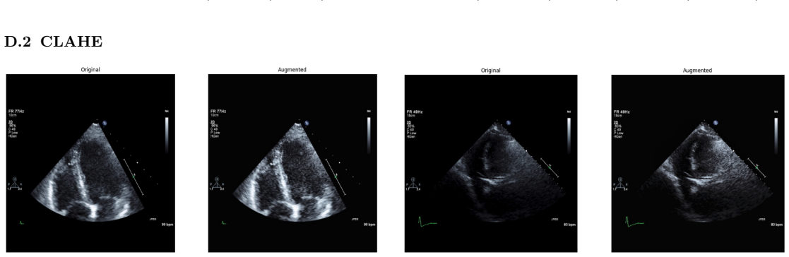
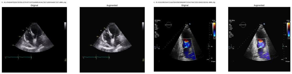
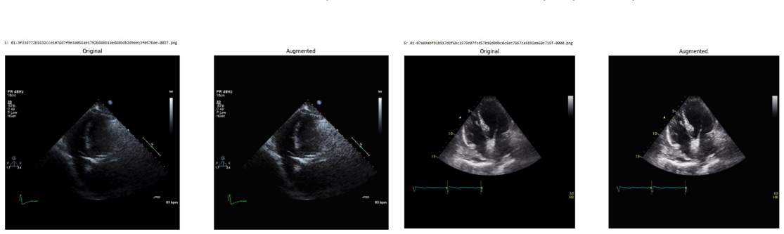
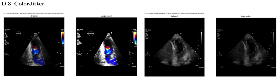
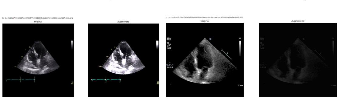
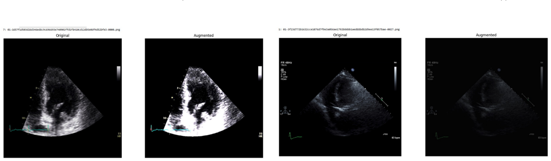
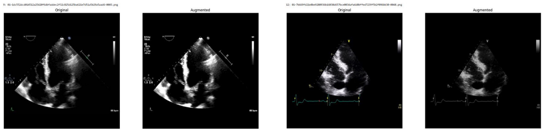
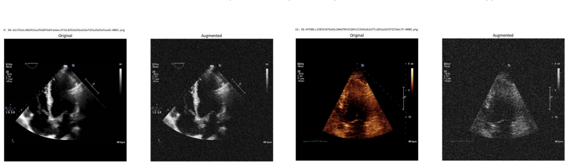
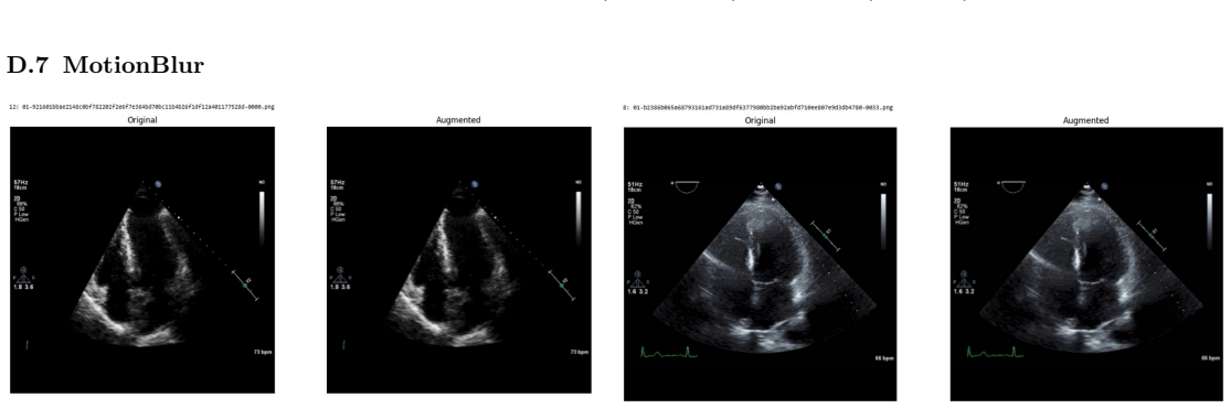
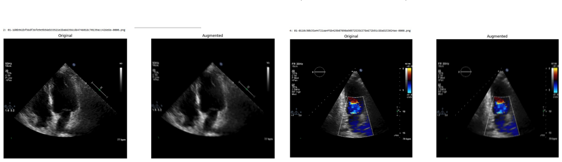
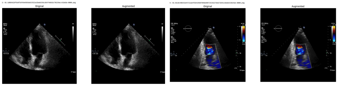
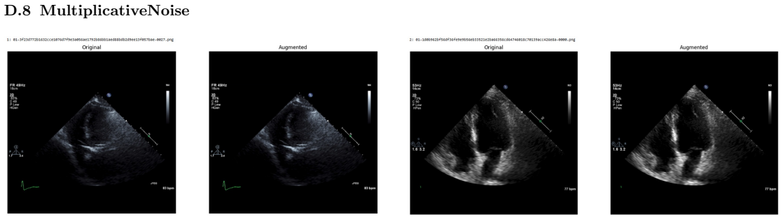
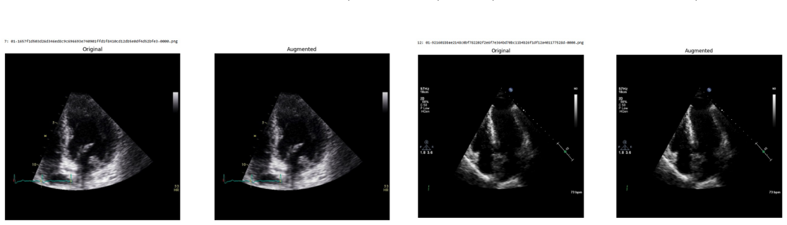
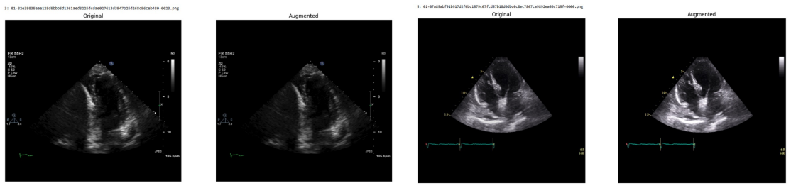
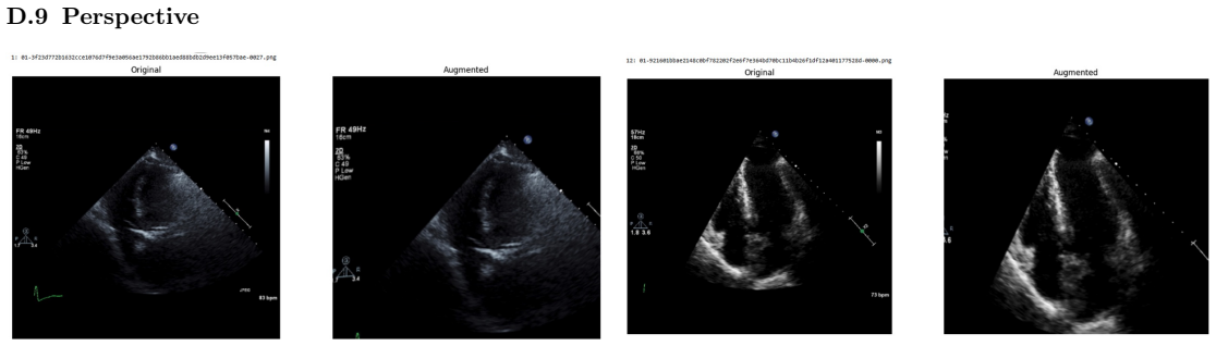
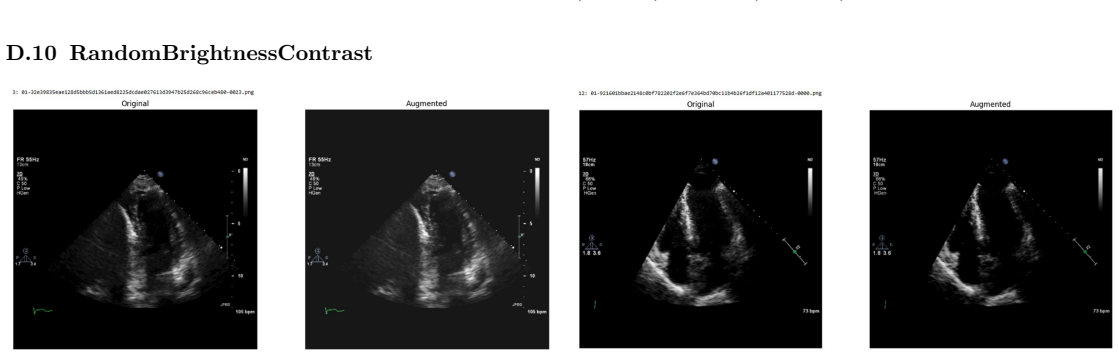
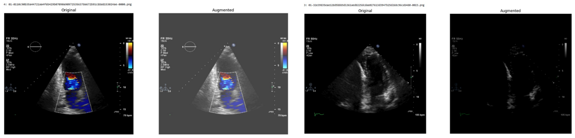
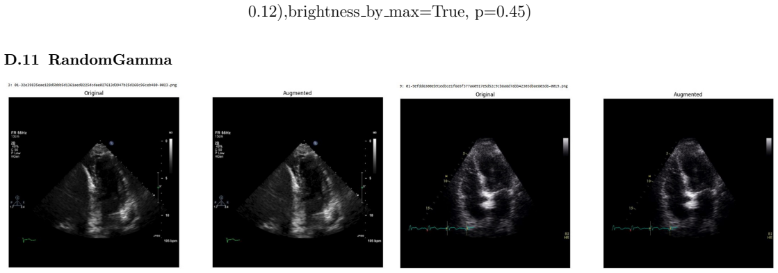
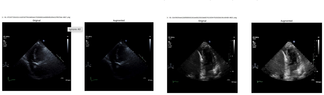
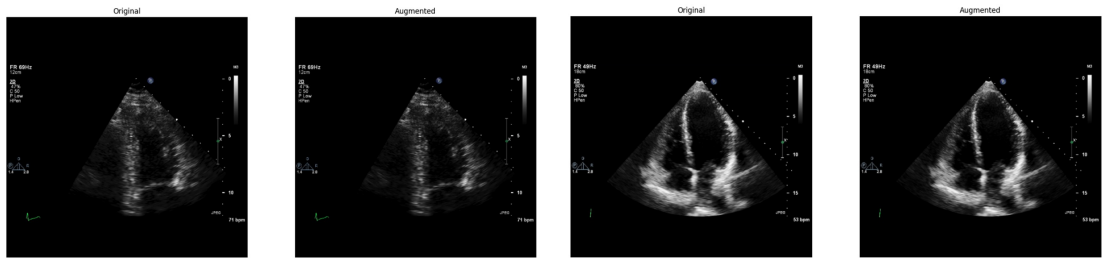
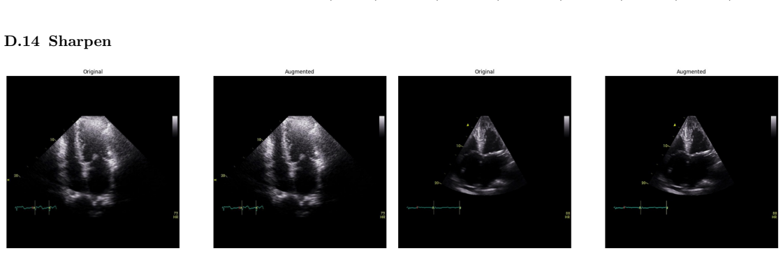
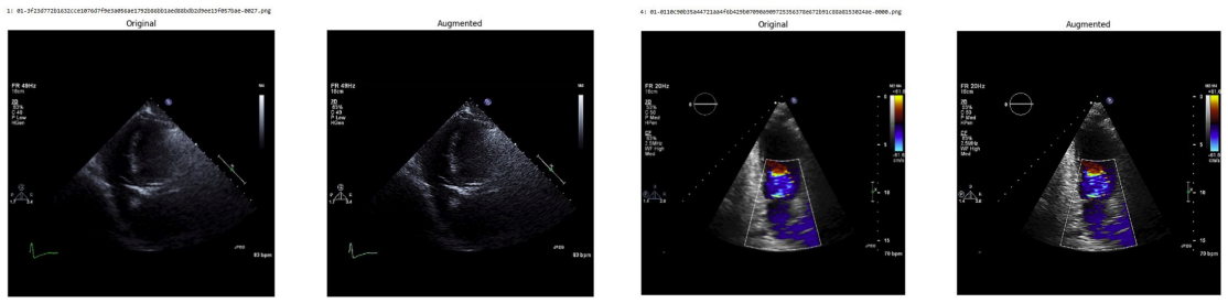
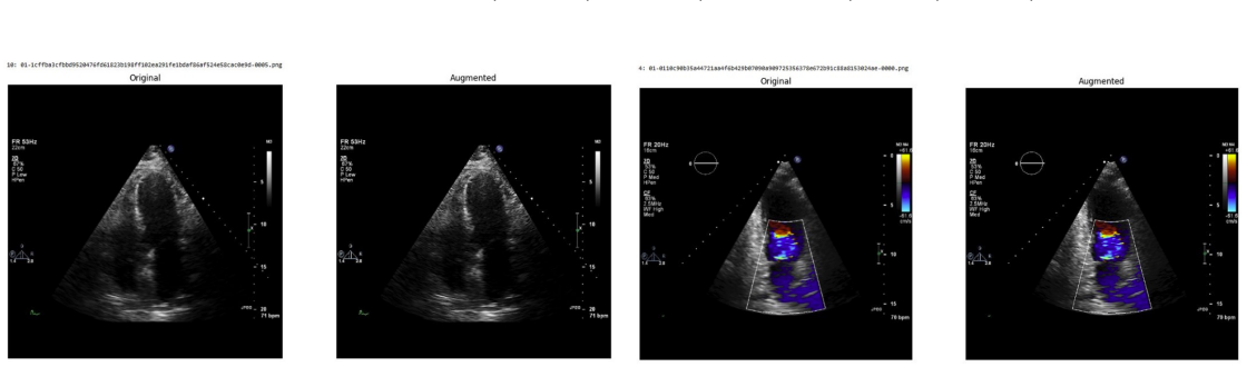
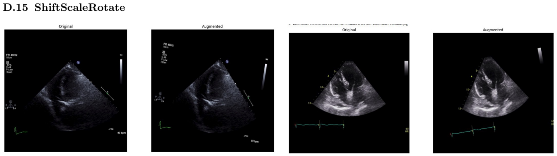
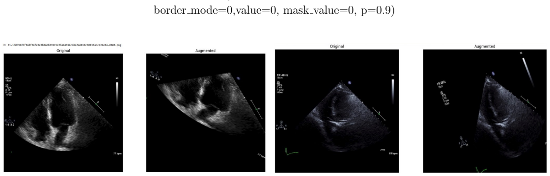
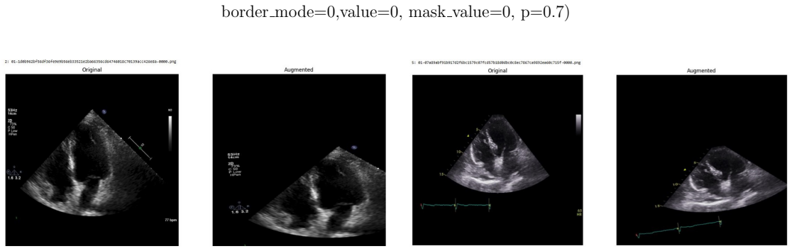
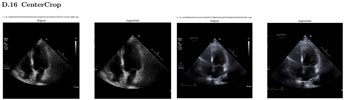
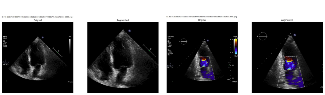
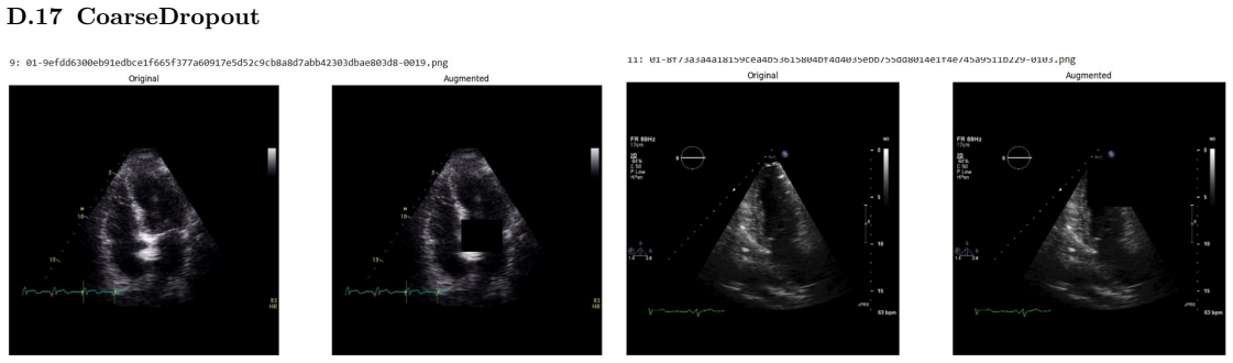
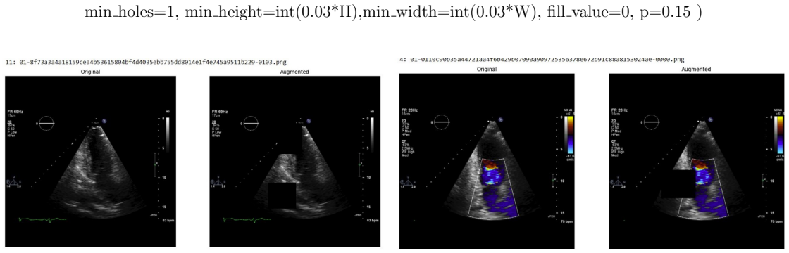
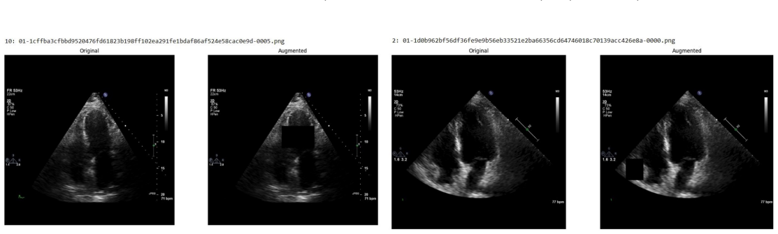
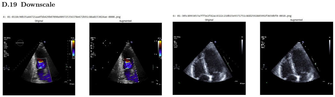
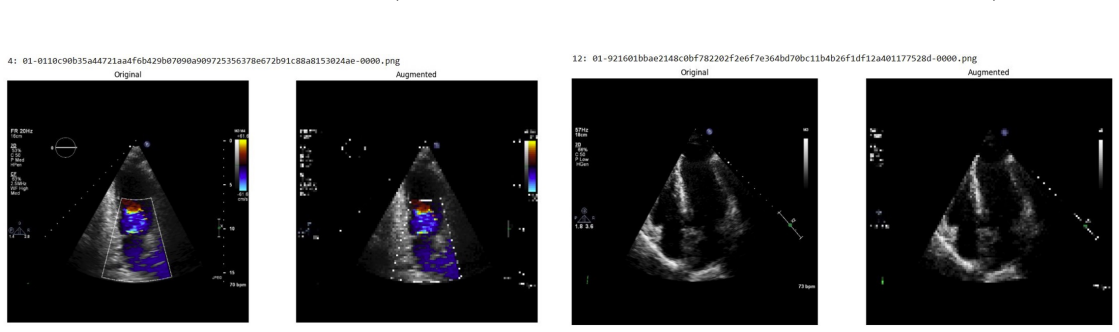
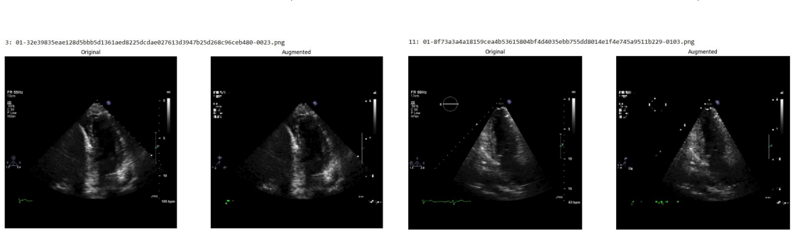
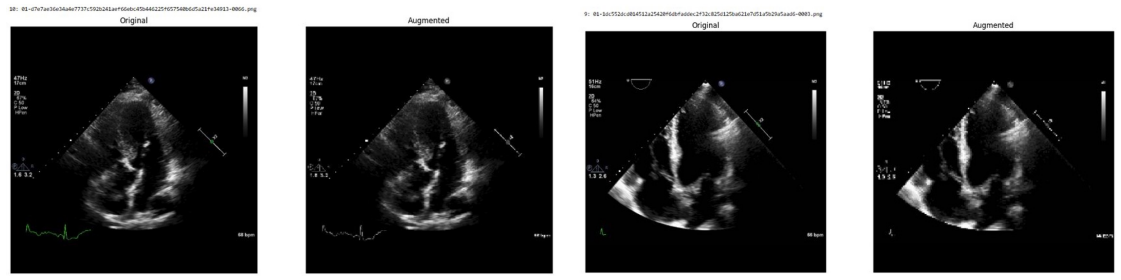
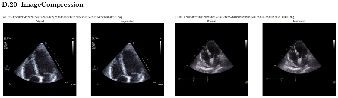
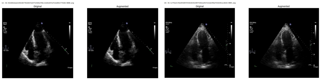
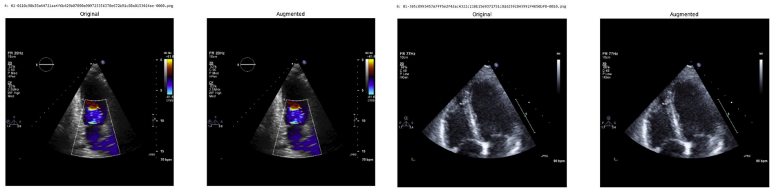
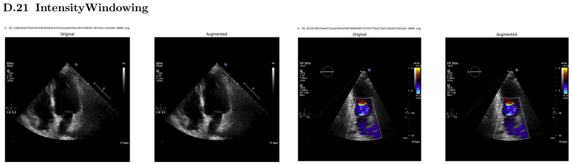
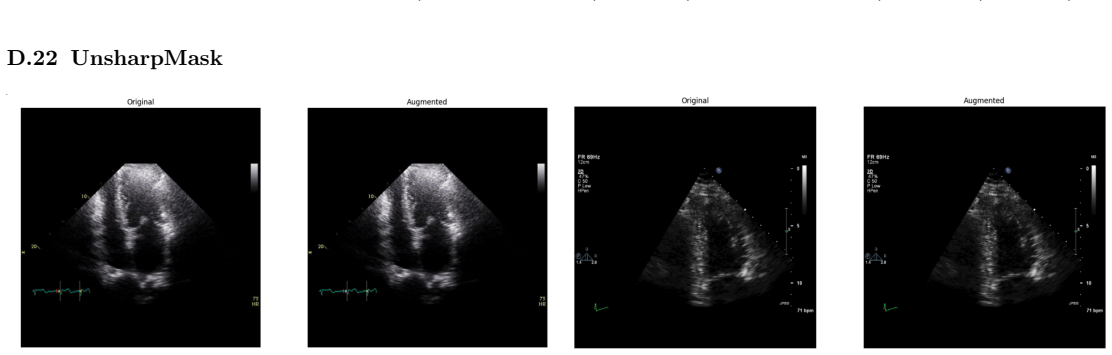
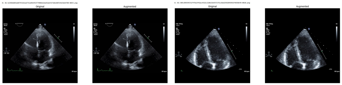
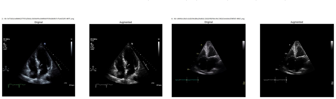
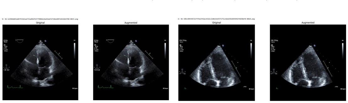
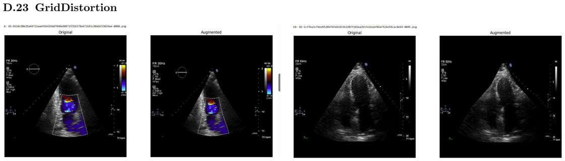
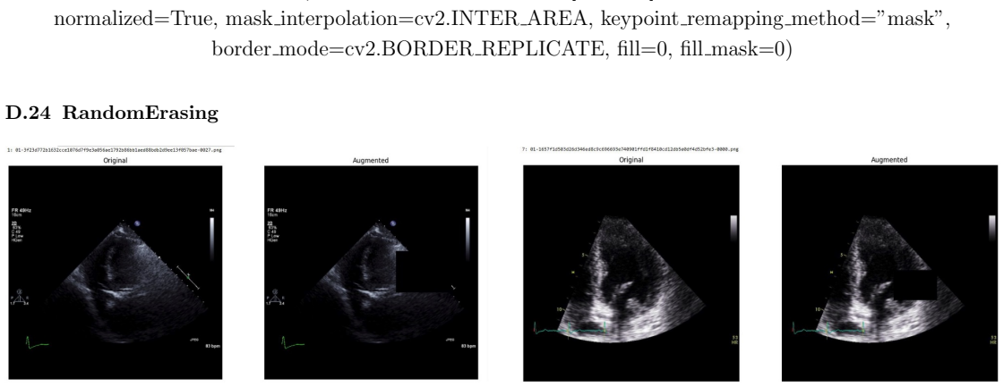
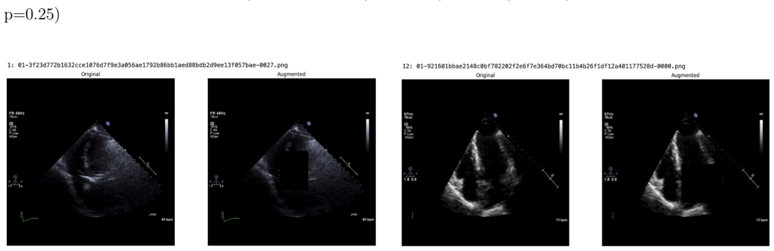
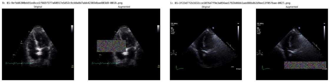
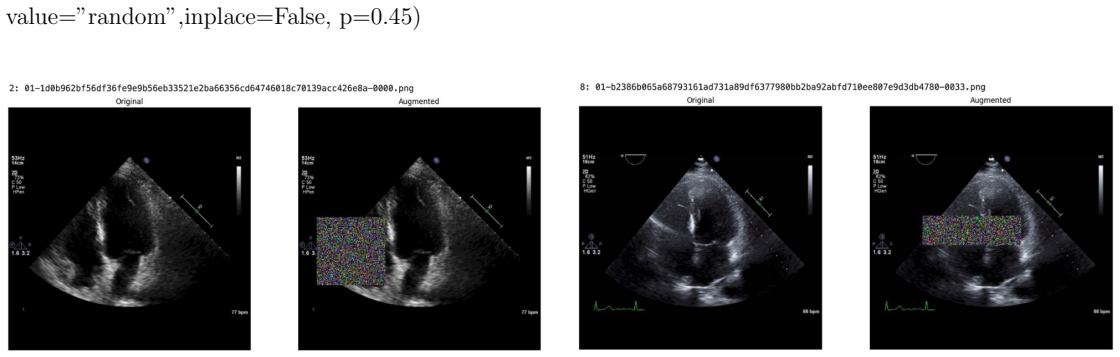
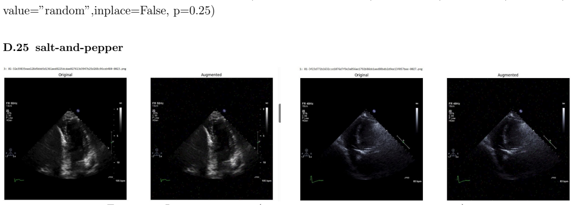
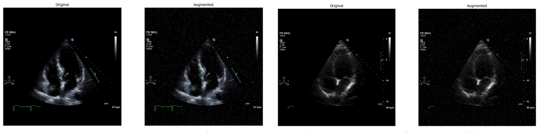
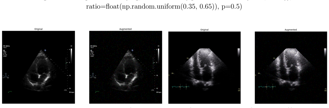
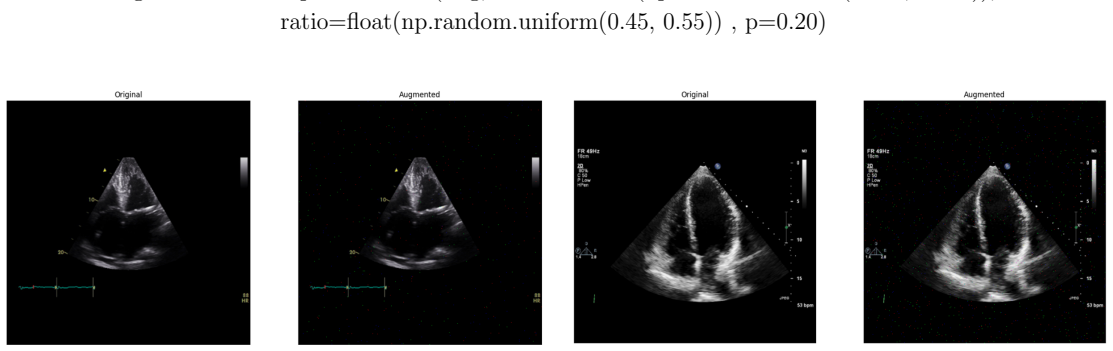
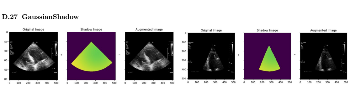
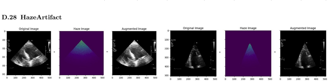
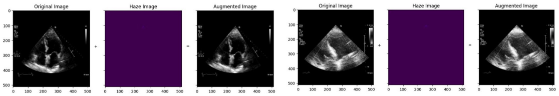
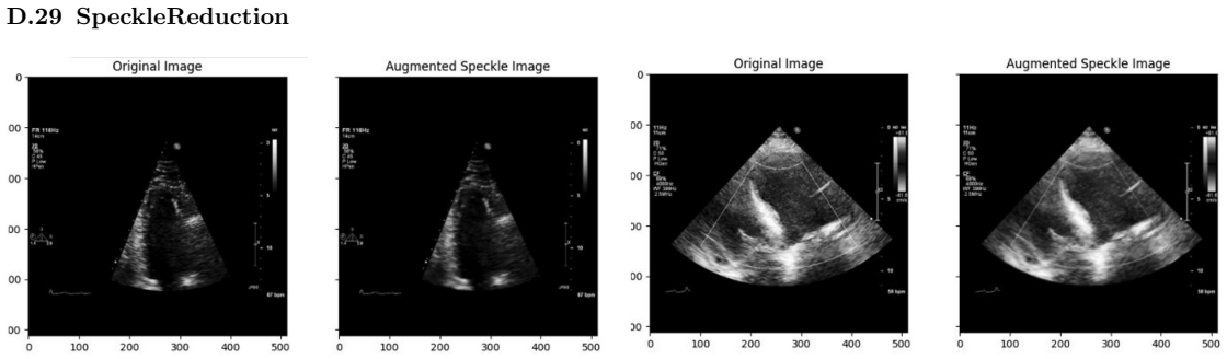
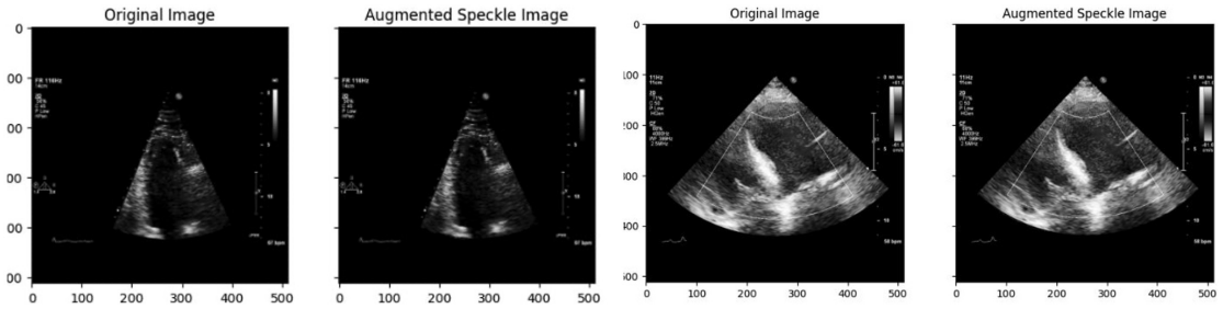
Deep learning models for echocardiography segmentation often struggle to generalise across institutions, scanners, and patient populations, where collecting large, consistently annotated datasets is infeasible. Data augmentation is widely used to improve the robustness of deep learning models; however, its role in enhancing cross-dataset generalisability in echocardiography remains insufficiently understood. This study presents a large-scale multi-dataset evaluation of 29 data augmentation techniques and their pairwise combinations for 2D left ventricular segmentation using a U-Net trained on Unity, CAMUS, and EchoNet Dynamic datasets. Each augmentation was explored under several hyperparameter settings and assessed through repeated runs using Dice and IoU in both in-domain and cross-dataset scenarios, with statistical significance quantified via independent t-tests. Results show that anatomically plausible geometric transformations, particularly affine, shift-scale-rotate, perspective, and random horizontal flip, substantially improve cross-dataset performance, whereas aggressive intensity- or artefact-based augmentations often degrade generalisability. Pairwise augmentation combinations outperform individual augmentations and show that moderate flip-centric combinations, especially random horizontal flip with affine, yield consistent gains across most transfer scenarios. These findings provide empirically grounded guidance for designing augmentation policies that enhance the robustness and transferability of echocardiography segmentation models.
Editorial analysis
A structured set of objections, weighed in public.
Referee Report
Summary. The manuscript conducts a large-scale evaluation of 29 data augmentation techniques and all their pairwise combinations for 2D left-ventricular segmentation with a U-Net. Training and testing are performed on the Unity, CAMUS and EchoNet-Dynamic datasets, with performance measured by Dice and IoU in both in-domain and cross-dataset settings. Repeated runs and independent t-tests are used to identify that anatomically plausible geometric transforms (affine, shift-scale-rotate, perspective, random horizontal flip) improve cross-dataset generalisability while aggressive intensity- or artefact-based augmentations degrade it, and that moderate flip-centric pairwise combinations yield the most consistent gains.
Significance. If the statistical claims survive correction for multiple testing and the experimental details are fully reported, the work supplies empirically grounded, practical guidance for augmentation policy design in echocardiography segmentation—an area where domain shift remains a central obstacle. The breadth of the augmentation sweep and the explicit cross-dataset protocol constitute a clear methodological contribution.
major comments (2)
- [Results] Results / Statistical analysis: The central claims rest on statistical significance obtained from a large number of independent t-tests performed across 29 augmentations, multiple hyper-parameter settings per augmentation, repeated runs, and all pairwise combinations. No correction for multiple comparisons (Bonferroni, Holm, or FDR) is mentioned. This directly affects which specific geometric transforms can be confidently declared beneficial or detrimental for generalisability.
- [Methods] Methods: Hyper-parameter ranges, exact implementation details for each of the 29 augmentations, and complete numerical results tables (including per-run Dice/IoU values) are not supplied. Without these, independent verification of the reported cross-dataset improvements is impossible.
minor comments (1)
- [Abstract] The abstract and results text would benefit from a concise statement of the total number of statistical tests performed so that readers can immediately appreciate the multiple-testing burden.
Simulated Author's Rebuttal
We thank the referee for their constructive and detailed review. We address each major comment below and outline the changes we will implement to enhance the statistical robustness and reproducibility of the manuscript.
read point-by-point responses
-
Referee: [Results] Results / Statistical analysis: The central claims rest on statistical significance obtained from a large number of independent t-tests performed across 29 augmentations, multiple hyper-parameter settings per augmentation, repeated runs, and all pairwise combinations. No correction for multiple comparisons (Bonferroni, Holm, or FDR) is mentioned. This directly affects which specific geometric transforms can be confidently declared beneficial or detrimental for generalisability.
Authors: We acknowledge that the large number of t-tests performed raises a legitimate issue of multiple comparisons. Our primary conclusions, however, are grounded in consistent performance patterns observed across independent datasets and augmentation families, rather than isolated p-values. In the revised manuscript we will apply Bonferroni correction to all reported tests, present the adjusted p-values, and explicitly state which geometric augmentations retain statistical support after correction. We will also clarify that practical recommendations are informed by both significance and effect size consistency. revision: yes
-
Referee: [Methods] Methods: Hyper-parameter ranges, exact implementation details for each of the 29 augmentations, and complete numerical results tables (including per-run Dice/IoU values) are not supplied. Without these, independent verification of the reported cross-dataset improvements is impossible.
Authors: We agree that these details are essential for reproducibility. The revised manuscript will expand the Methods section to list all 29 augmentations together with their explored hyper-parameter ranges and exact Albumentations implementations. A new supplementary section will contain full results tables reporting mean and standard deviation of Dice and IoU for every setting and run. Raw per-run values will be deposited in a public repository linked from the paper. revision: yes
- Whether every individual statistical claim will remain significant after Bonferroni correction, which requires re-analysis of the complete set of raw experimental results.
Circularity Check
No circularity: purely empirical evaluation of augmentations
full rationale
The paper performs an experimental study training U-Net models on Unity, CAMUS, and EchoNet Dynamic datasets, testing 29 augmentations and their pairwise combinations under multiple hyperparameters with repeated runs, then measuring Dice/IoU in in-domain and cross-dataset settings with independent t-tests. No equations, derivations, fitted parameters presented as predictions, or self-citations that bear the central load are present; all claims reduce directly to observed performance differences rather than any self-referential construction or renaming of inputs.
Axiom & Free-Parameter Ledger
free parameters (1)
- augmentation hyperparameters
axioms (1)
- domain assumption The selected datasets capture sufficient real-world scanner and population variability for cross-dataset evaluation.
Reference graph
Works this paper leans on
-
[1]
Islam, T., Hafiz, M. S., Jim, J. R., Kabir, M. M., and Mridha, M., “A systematic review of deep learning data augmentation in medical imaging: Recent advances and future research directions,”Healthcare Analytics5, 100340 (June 2024)
work page 2024
-
[2]
Wodzinski, M., Kwarciak, K., Daniol, M., and Hemmerling, D., “Improving deep learning-based au- tomatic cranial defect reconstruction by heavy data augmentation: From image registration to latent diffusion models,”Computers in Biology and Medicine182, 109129 (Nov. 2024)
work page 2024
-
[3]
A Com- prehensive Survey on Data Augmentation,
Wang, Z., Wang, P., Liu, K., Wang, P., Fu, Y., Lu, C.-T., Aggarwal, C. C., Pei, J., and Zhou, Y., “A Com- prehensive Survey on Data Augmentation,”IEEE Transactions on Knowledge and Data Engineering38, 47–66 (Jan. 2026)
work page 2026
-
[4]
Revisiting Data Augmentation for Ultrasound Images,
Tupper, A. and Gagn´ e, C., “Revisiting Data Augmentation for Ultrasound Images,” (2025). Version Number: 2
work page 2025
-
[5]
Image Data Augmentation Approaches: A Comprehensive Survey and Future Directions,
Kumar, T., Brennan, R., Mileo, A., and Bendechache, M., “Image Data Augmentation Approaches: A Comprehensive Survey and Future Directions,”IEEE Access12, 187536–187571 (2024)
work page 2024
-
[6]
Data Augmentation in Classification and Segmentation: A Survey and New Strategies,
Alomar, K., Aysel, H. I., and Cai, X., “Data Augmentation in Classification and Segmentation: A Survey and New Strategies,”Journal of Imaging9, 46 (Feb. 2023)
work page 2023
-
[7]
Medical image data augmentation: techniques, comparisons and interpretations,
Goceri, E., “Medical image data augmentation: techniques, comparisons and interpretations,”Artificial Intelligence Review56, 12561–12605 (Nov. 2023). 29
work page 2023
-
[8]
Segment anything model for medical image analysis: An experimental study,
Mazurowski, M. A., Dong, H., Gu, H., Yang, J., Konz, N., and Zhang, Y., “Segment anything model for medical image analysis: An experimental study,”Medical Image Analysis89, 102918 (Oct. 2023)
work page 2023
-
[9]
Segment anything in medical images,
Ma, J., He, Y., Li, F., Han, L., You, C., and Wang, B., “Segment anything in medical images,”Nature Communications15, 654 (Jan. 2024)
work page 2024
-
[10]
Contrastive Pretraining for Echocardiography Segmentation with Limited Data,
Saeed, M., Muhtaseb, R., and Yaqub, M., “Contrastive Pretraining for Echocardiography Segmentation with Limited Data,” (2022). Version Number: 3
work page 2022
-
[11]
Holste, G., Oikonomou, E. K., Mortazavi, B. J., Wang, Z., and Khera, R., “Efficient deep learning-based automated diagnosis from echocardiography with contrastive self-supervised learning,”Communications Medicine4, 133 (July 2024)
work page 2024
-
[12]
Guo, Z., Zhang, Y., Qiu, Z., Dong, S., He, S., Gao, H., Zhang, J., Chen, Y., He, B., Kong, Z., Qiu, Z., Li, Y., and Li, C., “An improved contrastive learning network for semi-supervised multi-structure segmentation in echocardiography,”Frontiers in Cardiovascular Medicine10, 1266260 (Sept. 2023)
work page 2023
-
[13]
Varghese, A. P., Naik, S., Asrar Up Haq Andrabi, S., Luharia, A., and Tivaskar, S., “Enhancing Radio- logical Diagnosis: A Comprehensive Review of Image Quality Assessment and Optimization Strategies,” Cureus(June 2024)
work page 2024
-
[14]
Bone shadow segmentation from ultrasound data for orthopedic surgery using GAN,
Alsinan, A. Z., Patel, V. M., and Hacihaliloglu, I., “Bone shadow segmentation from ultrasound data for orthopedic surgery using GAN,”International Journal of Computer Assisted Radiology and Surgery15, 1477–1485 (Sept. 2020)
work page 2020
-
[15]
UltraAugment: Fan-shape and Artifact- based Data Augmentation for 2D Ultrasound Images,
Ramakers, F., Vercauteren, T., Deprest, J., and Williams, H., “UltraAugment: Fan-shape and Artifact- based Data Augmentation for 2D Ultrasound Images,” in [2024 IEEE/CVF Conference on Computer Vision and Pattern Recognition Workshops (CVPRW)], 2422–2431, IEEE, Seattle, WA, USA (June 2024)
work page 2024
-
[16]
Moinuddin, M., Khan, S., Alsaggaf, A. U., Abdulaal, M. J., Al-Saggaf, U. M., and Ye, J. C., “Medical ul- trasound image speckle reduction and resolution enhancement using texture compensated multi-resolution convolution neural network,”Frontiers in Physiology13, 961571 (Nov. 2022)
work page 2022
-
[17]
Boumeridja, H., Ammar, M., Alzubaidi, M., Mahmoudi, S., Benamer, L. N., Agus, M., Househ, M., Lekadir, K., and El Habib Daho, M., “Enhancing fetal ultrasound image quality and anatomical plane recognition in low-resource settings using super-resolution models,”Scientific Reports15, 8376 (Mar. 2025)
work page 2025
-
[18]
Ultrasam: a foundation model for ul- trasound using large open-access segmentation datasets,
Meyer, A., Murali, A., Zarin, F., Mutter, D., and Padoy, N., “Ultrasam: a foundation model for ul- trasound using large open-access segmentation datasets,”International Journal of Computer Assisted Radiology and Surgery(Sept. 2025)
work page 2025
-
[19]
Sfakianakis, C., Simantiris, G., and Tziritas, G., “GUDU: Geometrically-constrained Ultrasound Data augmentation in U-Net for echocardiography semantic segmentation,”Biomedical Signal Processing and Control82, 104557 (Apr. 2023)
work page 2023
-
[20]
Guo, B., Lu, D., Szumel, G., Gui, R., Wang, T., Konz, N., and Mazurowski, M. A., “The impact of scanner domain shift on deep learning performance in medical imaging: an experimental study,”arXiv preprint arXiv:2409.04368(2024)
-
[21]
Semi-supervised Active Learning for Left Ventricle Segmentation in Echocardiography,
Alajrami, E., DadashiSerej, N., Jevsikov, J., Fernandes, P., Abdi, A., Ufumaka, I., Francis, D. P., and Zolgharni, M., “Semi-supervised Active Learning for Left Ventricle Segmentation in Echocardiography,” in [Medical Imaging with Deep Learning], 30
-
[22]
Self-supervised learning for label-free segmen- tation in cardiac ultrasound,
Ferreira, D. L., Lau, C., Salaymang, Z., and Arnaout, R., “Self-supervised learning for label-free segmen- tation in cardiac ultrasound,”Nature Communications16, 4070 (Apr. 2025)
work page 2025
-
[23]
A self-supervised semi-supervised echocardiographic video left ventricle segmen- tation method,
Wang, T. and Dai, Q., “A self-supervised semi-supervised echocardiographic video left ventricle segmen- tation method,”Biomedical Signal Processing and Control101, 107211 (Mar. 2025)
work page 2025
-
[24]
Consensus-guided evaluation of self-supervised learning in echocardiographic segmentation,
Naidoo, P., Fernandes, P., Dadashi Serej, N., Manisty, C. H., Shun-Shin, M. J., Francis, D. P., and Zol- gharni, M., “Consensus-guided evaluation of self-supervised learning in echocardiographic segmentation,” Computers in Biology and Medicine198, 111148 (Nov. 2025)
work page 2025
-
[25]
Rethinking Self-Supervised Semantic Segmentation: Achieving End-to-End Segmentation,
Liu, Y., Zeng, J., Tao, X., and Fang, G., “Rethinking Self-Supervised Semantic Segmentation: Achieving End-to-End Segmentation,”IEEE Transactions on Pattern Analysis and Machine Intelligence46, 10036– 10046 (Dec. 2024)
work page 2024
-
[26]
A Survey on Self-Supervised Learning: Algorithms, Applications, and Future Trends,
Gui, J., Chen, T., Zhang, J., Cao, Q., Sun, Z., Luo, H., and Tao, D., “A Survey on Self-Supervised Learning: Algorithms, Applications, and Future Trends,”IEEE Transactions on Pattern Analysis and Machine Intelligence46, 9052–9071 (Dec. 2024)
work page 2024
-
[27]
Contrastive Learning for View Classification of Echocardiograms,
Chartsias, A., Gao, S., Mumith, A., Oliveira, J., Bhatia, K., Kainz, B., and Beqiri, A., “Contrastive Learning for View Classification of Echocardiograms,” in [Simplifying Medical Ultrasound], Noble, J. A., Aylward, S., Grimwood, A., Min, Z., Lee, S.-L., and Hu, Y., eds.,12967, 149–158, Springer International Publishing, Cham (2021). Series Title: Lecture...
work page 2021
-
[28]
Segmenting Cardiac Ultrasound Videos Using Self-Supervised Learning,
Lamoureux, E., Ayromlou, S., Ahmadi Amiri, S. N., and Rhodin, H., “Segmenting Cardiac Ultrasound Videos Using Self-Supervised Learning,” in [2023 45th Annual International Conference of the IEEE Engineering in Medicine & Biology Society (EMBC)], 1–7, IEEE, Sydney, Australia (July 2023)
work page 2023
-
[29]
EchoFM: Foundation Model for Generalizable Echocardiogram Analysis,
Kim, S., Jin, P., Song, S., Chen, C., Li, Y., Ren, H., Li, X., Liu, T., and Li, Q., “EchoFM: Foundation Model for Generalizable Echocardiogram Analysis,”IEEE Transactions on Medical Imaging44, 4049– 4062 (Oct. 2025)
work page 2025
-
[30]
Integrating Deep Metric Learning with Coreset for Active Learning in 3D Segmentation,
Vepa, A. M., Yang, Z., Choi, A., Joo, J., Scalzo, F., and Sun, Y., “Integrating Deep Metric Learning with Coreset for Active Learning in 3D Segmentation,” (2024). Version Number: 1
work page 2024
-
[31]
Wang, H., Jin, Q., Du, X., Wang, L., Guo, Q., Li, H., Wang, M., and Song, Z., “MDAL: Modality- difference-based active learning for multimodal medical image analysis via contrastive learning and point- wise mutual information,”Computerized Medical Imaging and Graphics123, 102544 (July 2025)
work page 2025
-
[32]
Zhang, J., Zhang, S., Shen, X., Lukasiewicz, T., and Xu, Z., “Multi-ConDoS: Multimodal Contrastive Domain Sharing Generative Adversarial Networks for Self-Supervised Medical Image Segmentation,” IEEE Transactions on Medical Imaging43, 76–95 (Jan. 2024)
work page 2024
-
[33]
EchoGNN with Contrastive Learning,
Kondori, N., Fung, A., and Goco, J. A. D., “EchoGNN with Contrastive Learning,”
-
[34]
RadImageNet: An Open Radiologic Deep Learning Research Dataset for Effective Transfer Learning,
Mei, X., Liu, Z., Robson, P. M., Marinelli, B., Huang, M., Doshi, A., Jacobi, A., Cao, C., Link, K. E., Yang, T., Wang, Y., Greenspan, H., Deyer, T., Fayad, Z. A., and Yang, Y., “RadImageNet: An Open Radiologic Deep Learning Research Dataset for Effective Transfer Learning,”Radiology: Artificial Intel- ligence4, e210315 (Sept. 2022)
work page 2022
-
[35]
Eche, T., Schwartz, L. H., Mokrane, F.-Z., and Dercle, L., “Toward Generalizability in the Deployment of Artificial Intelligence in Radiology: Role of Computation Stress Testing to Overcome Underspecification,” Radiology: Artificial Intelligence3, e210097 (Nov. 2021). 31
work page 2021
-
[36]
Active learning for left ventricle segmentation in echocardiography,
Alajrami, E., Ng, T., Jevsikov, J., Naidoo, P., Fernandes, P., Azarmehr, N., Dinmohammadi, F., Shun- shin, M. J., Dadashi Serej, N., Francis, D. P., and Zolgharni, M., “Active learning for left ventricle segmentation in echocardiography,”Computer Methods and Programs in Biomedicine248, 108111 (May 2024)
work page 2024
-
[37]
Qu, L., Jin, Q., Fu, K., Wang, M., and Song, Z., “Rethinking deep active learning for medical image segmentation: A diffusion and angle-based framework,”Biomedical Signal Processing and Control96, 106493 (Oct. 2024)
work page 2024
-
[38]
Two-View Left Ventricular Segmentation and Ejection Fraction Estimation in 2D Echocardiograms.,
Tabuco, F. C. A., Magno, J. D. A., Orillaza Jr, N. S., Domingo, R. A. V., and Naval, P. C., “Two-View Left Ventricular Segmentation and Ejection Fraction Estimation in 2D Echocardiograms.,” in [BMVC], 176 (2022)
work page 2022
-
[39]
Fast and accurate view classification of echocar- diograms using deep learning,
Madani, A., Arnaout, R., Mofrad, M., and Arnaout, R., “Fast and accurate view classification of echocar- diograms using deep learning,”npj Digital Medicine1, 6 (Mar. 2018)
work page 2018
-
[40]
Chen, S.-H., Weng, K.-P., Hsieh, K.-S., Chen, Y.-H., Shih, J.-H., Li, W.-R., Zhang, R.-Y., Chen, Y.-C., Tsai, W.-R., and Kao, T.-Y., “Optimizing Object Detection Algorithms for Congenital Heart Diseases in Echocardiography: Exploring Bounding Box Sizes and Data Augmentation Techniques,”Reviews in Cardiovascular Medicine25, 335 (Sept. 2024)
work page 2024
-
[41]
Unsupervised Echocardiography Registration Through Patch-Based MLPs and Transformers,
Wang, Z., Yang, Y., Sermesant, M., and Delingette, H., “Unsupervised Echocardiography Registration Through Patch-Based MLPs and Transformers,” in [Statistical Atlases and Computational Models of the Heart. Regular and CMRxMotion Challenge Papers], Camara, O., Puyol-Ant´ on, E., Qin, C., Sermesant, M., Suinesiaputra, A., Wang, S., and Young, A., eds.,13593...
work page 2022
-
[42]
Artificial intelligence-based classification of echocardiographic views,
Naser, J. A., Lee, E., Pislaru, S. V., Tsaban, G., Malins, J. G., Jackson, J. I., Anisuzzaman, D. M., Rostami, B., Lopez-Jimenez, F., Friedman, P. A., Kane, G. C., Pellikka, P. A., and Attia, Z. I., “Artificial intelligence-based classification of echocardiographic views,”European Heart Journal - Digital Health5, 260–269 (May 2024)
work page 2024
-
[43]
Generative augmentations for improved cardiac ultrasound segmentation using diffusion models,
Van De Vyver, G., Lenz, A. T., Smistad, E., Olaisen, S. H., Grenne, B., Holte, E., Dalen, H., and Løvstakken, L., “Generative augmentations for improved cardiac ultrasound segmentation using diffusion models,”Scientific Reports15, 38013 (Oct. 2025)
work page 2025
-
[44]
Annotation Cost Minimization for Ultrasound Image Segmentation using Cross-domain Transfer Learning,
Monkam, P., Jin, S., and Lu, W., “Annotation Cost Minimization for Ultrasound Image Segmentation using Cross-domain Transfer Learning,”IEEE Journal of Biomedical and Health Informatics, 1–11 (2023)
work page 2023
-
[45]
Myocardial Function Imaging in Echocardiography Using Deep Learning,
Ostvik, A., Salte, I. M., Smistad, E., Nguyen, T. M., Melichova, D., Brunvand, H., Haugaa, K., Edvard- sen, T., Grenne, B., and Lovstakken, L., “Myocardial Function Imaging in Echocardiography Using Deep Learning,”IEEE Transactions on Medical Imaging40, 1340–1351 (May 2021)
work page 2021
-
[46]
Li, X., Wang, Y., Zhao, Y., and Wei, Y., “Fast Speckle Noise Suppression Algorithm in Breast Ultrasound Image Using Three-Dimensional Deep Learning,”Frontiers in Physiology13, 880966 (Apr. 2022)
work page 2022
-
[47]
Comprehensive echocardiogram evaluation with view primed vision language AI,
Vukadinovic, M., Chiu, I.-M., Tang, X., Yuan, N., Chen, T.-Y., Cheng, P., Li, D., Cheng, S., He, B., and Ouyang, D., “Comprehensive echocardiogram evaluation with view primed vision language AI,”Nature (Nov. 2025). 32
work page 2025
-
[48]
Smistad, E., Johansen, K. F., Iversen, D. H., and Reinertsen, I., “Highlighting nerves and blood vessels for ultrasound-guided axillary nerve block procedures using neural networks,”Journal of Medical Imaging5, 1 (Nov. 2018)
work page 2018
-
[49]
Video-based AI for beat-to-beat assessment of cardiac function,
Ouyang, D., He, B., Ghorbani, A., Yuan, N., Ebinger, J., Langlotz, C. P., Heidenreich, P. A., Harrington, R. A., Liang, D. H., Ashley, E. A., and Zou, J. Y., “Video-based AI for beat-to-beat assessment of cardiac function,”Nature580, 252–256 (Apr. 2020)
work page 2020
-
[50]
Ouyang, D., He, B., Ghorbani, A., Yuan, N., Ebinger, J., Langlotz, C. P., Heidenreich, P. A., Harrington, R. A., Liang, D. H., Ashley, E. A., and Zou, J. Y., “EchoNet-Dynamic,” (2020)
work page 2020
-
[51]
Deep Learning for Segmentation Using an Open Large-Scale Dataset in 2D Echocardiography,
Leclerc, S., Smistad, E., Pedrosa, J., Ostvik, A., Cervenansky, F., Espinosa, F., Espeland, T., Berg, E. A. R., Jodoin, P.-M., Grenier, T., Lartizien, C., Dhooge, J., Lovstakken, L., and Bernard, O., “Deep Learning for Segmentation Using an Open Large-Scale Dataset in 2D Echocardiography,”IEEE Trans- actions on Medical Imaging38, 2198–2210 (Sept. 2019)
work page 2019
-
[52]
Howard, J. P., Stowell, C. C., Cole, G. D., Ananthan, K., Demetrescu, C. D., Pearce, K., Rajani, R., Sehmi, J., Vimalesvaran, K., Kanaganayagam, G. S., et al., “Automated left ventricular dimension assessment using artificial intelligence developed and validated by a uk-wide collaborative,”Circulation: Cardiovascular Imaging14(5), e011951 (2021)
work page 2021
-
[53]
Echonet- dynamic: a large new cardiac motion video data resource for medical machine learning,
Ouyang, D., He, B., Ghorbani, A., Lungren, M. P., Ashley, E. A., Liang, D. H., and Zou, J. Y., “Echonet- dynamic: a large new cardiac motion video data resource for medical machine learning,”Conference on Neural Information Processing Systems (NeurIPS)33(2019)
work page 2019
-
[54]
Dsmri: domain shift analyzer for multi-center mri datasets,
Kushol, R., Wilman, A. H., Kalra, S., and Yang, Y.-H., “Dsmri: domain shift analyzer for multi-center mri datasets,”Diagnostics13(18), 2947 (2023)
work page 2023
-
[55]
Yan, W., Huang, L., Xia, L., Gu, S., Yan, F., Wang, Y., and Tao, Q., “Mri manufacturer shift and adaptation: increasing the generalizability of deep learning segmentation for mr images acquired with different scanners,”Radiology: Artificial Intelligence2(4), e190195 (2020)
work page 2020
-
[56]
A simple framework for contrastive learning of visual representations,
Chen, T., Kornblith, S., Norouzi, M., and Hinton, G., “A simple framework for contrastive learning of visual representations,” in [International conference on machine learning], 1597–1607, PmLR (2020)
work page 2020
-
[57]
Momentum contrast for unsupervised visual repre- sentation learning,
He, K., Fan, H., Wu, Y., Xie, S., and Girshick, R., “Momentum contrast for unsupervised visual repre- sentation learning,” in [Proceedings of the IEEE/CVF conference on computer vision and pattern recog- nition], 9729–9738 (2020)
work page 2020
-
[58]
Bootstrap your own latent-a new approach to self-supervised learning,
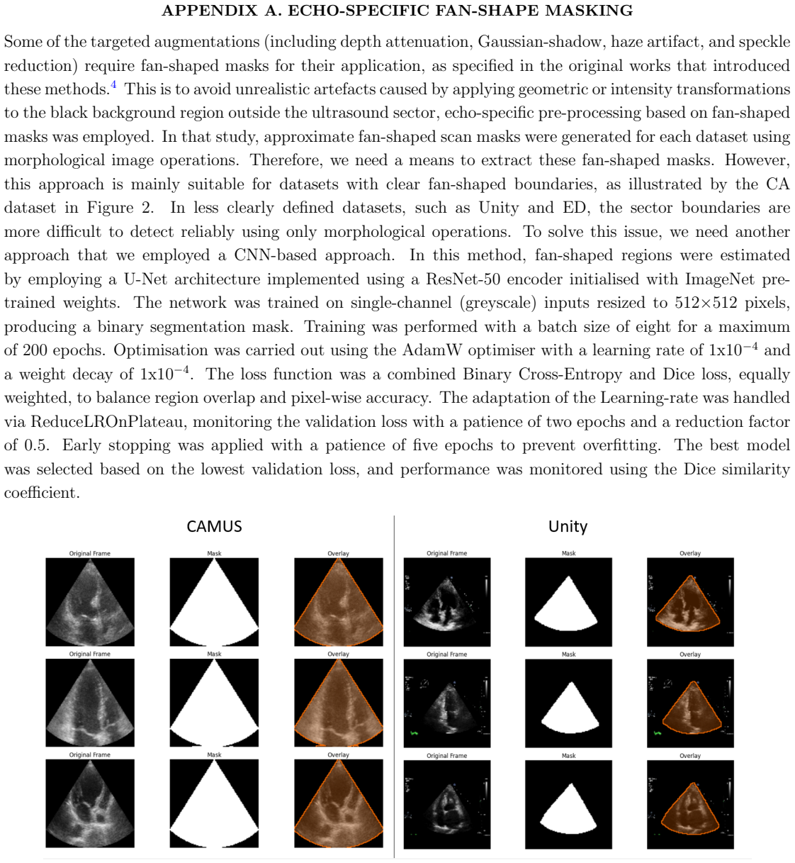
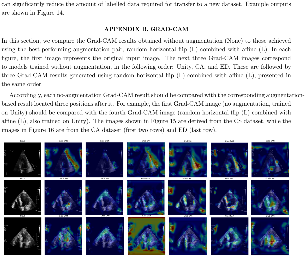
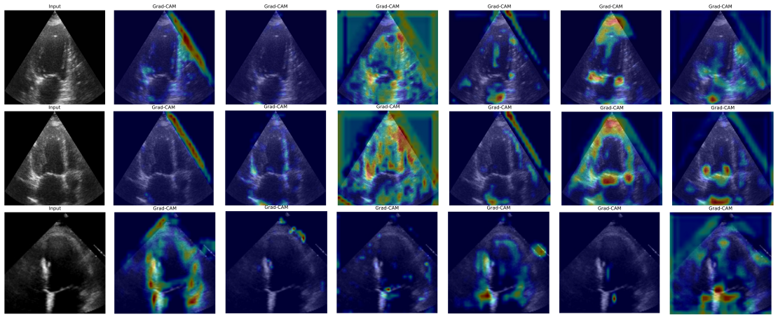
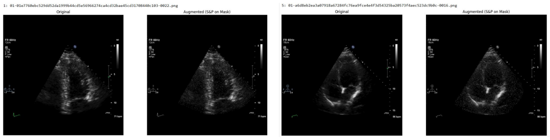
Grill, J.-B., Strub, F., Altch´ e, F., Tallec, C., Richemond, P., Buchatskaya, E., Doersch, C., Avila Pires, B., Guo, Z., Gheshlaghi Azar, M., et al., “Bootstrap your own latent-a new approach to self-supervised learning,”Advances in neural information processing systems33, 21271–21284 (2020). 33 APPENDIX A. ECHO-SPECIFIC FAN-SHAPE MASKING Some of the tar...
work page 2020
discussion (0)
Sign in with ORCID, Apple, or X to comment. Anyone can read and Pith papers without signing in.