REVIEW 4 major objections 5 minor 33 references
From level set evolution to threshold optimization: A grayscale level set framework for image segmentation
T0 review · 4 major / 5 minor · reviewed 2026-08-01 · deepseek-v4-flash
Pith's one-line read Once a degraded image is smoothed into a threshold-separable form, the paper proves, level-set segmentation reduces to picking a single gray-level cutoff — with no length regularization or PDE evolution.
desk verdict The optimality theorem is circular and the framework is essentially thresholding after denoising, but the incremental O(NS) threshold scan is a genuine speedup and the empirical observation is worth a second look. read the letter →
The pith
A machine-rendered reading of the paper's core claim, the machinery that carries it, and where it could break.
The reading
What carries the argument
Grayscale level set: the family Φ_c = {φ_c(x) = SDF(Γ_c) : c ∈ [Cmin, Cmax]}, where J is the smoothed image, Γ_c is the boundary of the superlevel set {J > c}, and SDF is the signed distance function (distance from each pixel to the contour, signed by which side it lies on). This family is a subspace of traditional level-set space and is the mechanism that converts curvature-driven PDE evolution into one-dimensional threshold optimization. Supporting it are the definition of a smooth image (bounded gradient plus threshold separability of the two regions), the co-area formula (which bounds the total arc length of candidate contours by L·|Ω|), and an incremental update algorithm that reuses co
What would settle it
Take a synthetic image whose two regions have overlapping intensity distributions even after strong denoising and bias correction, and check whether any threshold c satisfies sup_{Ω2} J < c < inf_{Ω1} J for the ground-truth partition. If no such threshold exists, or if the regularization-free fitting energy has a global minimizer that is not a threshold partition, Theorem 3.3.3 fails. Concretely, a two-Gaussian-mixture image with means separated by less than the combined standard deviations after optimal preprocessing would falsify the framework's central premise.
Extended reading notes
Core claim
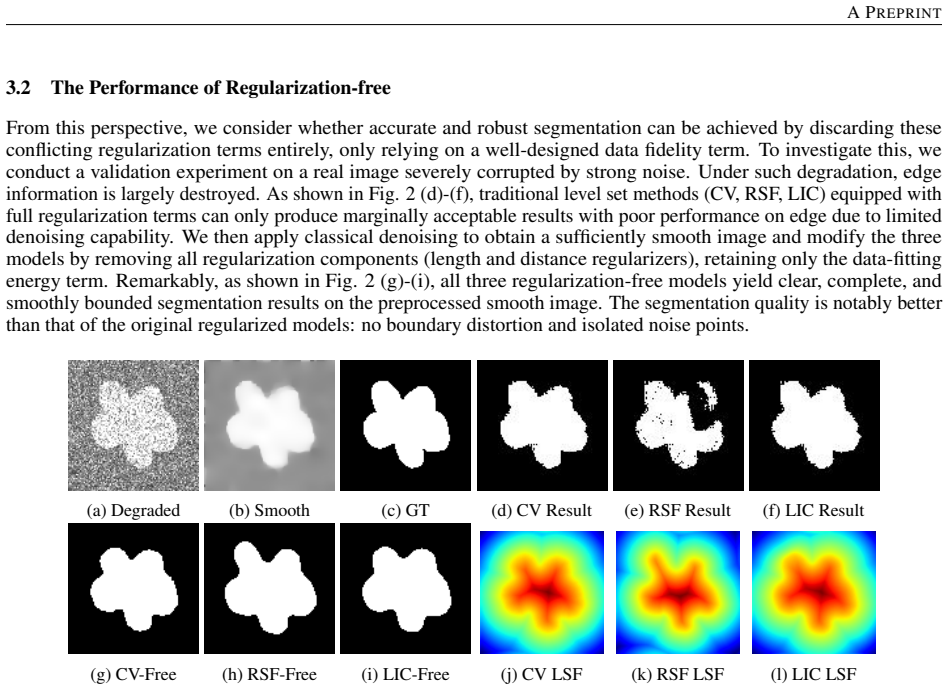
The central claim, stated as Theorem 3.3.3, is that on a smooth image satisfying the separation condition of Definition 3.3.1, the global minimum of the regularization-free fitting energy over threshold partitions equals the global minimum over all admissible two-region partitions. In other words, the optimal segmentation boundary can be represented as a level contour Γ_c = ∂{x : J(x) > c*} of the smoothed image, so the search for a level-set function can be compressed to the grayscale level set without loss of optimality. The paper further shows the length term conflicts with distance regularization (driving |∇φ| toward 0 while distance regularization drives it toward 1), and that on smooth
Load-bearing premise
The argument rests on the assumption that, after preprocessing, the object and background can be separated by a single gray-level cutoff, and that the true best two-region partition is one of those cutoffs — if a real image cannot be smoothed into that form without moving the boundary, the claimed equivalence between threshold search and full variational segmentation no longer holds.
Editorial extensions
If this is right
- Length regularization can be dropped from level-set segmentation after preprocessing, removing the conflicting dynamics between the length term and distance regularization.
- Segmentation cost becomes independent of threshold discretization: for an N-pixel image with kernel support S, the full threshold sweep costs O(N·S) instead of O(M·N·S), making large images far cheaper to segment.
- Because the optimal contour is found by a global threshold scan rather than curve evolution, results are insensitive to the initialization that trips iterative level-set methods.
- Preprocessing and segmentation decouple cleanly: the segmentation stage is unchanged regardless of which denoising or bias-correction operator produced the smooth image, as long as the separation condition holds.
- On images that meet the smoothness and separation assumptions, the variational segmentation problem is no longer a local-minima-prone evolution but a well-posed one-dimensional optimization with a global minimizer among threshold contours.
Reading between the lines
- If the equivalence holds broadly, classical variational segmentation could regain a speed advantage over deep networks on very large images, at the price of overlap accuracy on complex textured regions; the paper's own histopathology comparison hints at this trade-off, though the paper frames the result as a geometric benefit.
- The threshold-separability premise suggests a testable extension: the method could be viewed as histogram-mode analysis of the smoothed image, and extended to multi-phase segmentation by searching over multiple thresholds — a direction the paper lists as future work.
- The advertised complexity gain depends on the kernel support S remaining small; for very large smoothing scales the local updates become global, so the speedup is most meaningful for localized fitting kernels.
- One could stress-test the central assumption by measuring, after each preprocessing operator, the intensity-range gap between ground-truth regions; images with no gap should directly predict failures, making the assumption a diagnostic tool rather than only a hypothesis.
Editorial analysis
A structured set of objections, weighed in public.
Referee Report
Summary. The paper proposes a "grayscale level set" segmentation framework that, after a preprocessing step, replaces PDE-based level-set evolution by a one-dimensional threshold search. The authors claim that under a new definition of smooth images the length regularization term is unnecessary, that the optimal solution of a regularization-free fitting energy is representable in the grayscale-level-set space, and that an incremental update reduces complexity from O(M·N·S) to O(N·S). Experiments on synthetic and real images report competitive accuracy and large speedups.
Significance. If the theoretical claims were valid, the framework would offer a genuinely fast and simple alternative to variational level-set segmentation for degraded images, and the decoupling of preprocessing from segmentation would be practically attractive. The incremental threshold update in Algorithm 1 is a clear algorithmic idea, and the experimental results on several datasets (WBC, BrainWeb, DIAS, MoNuSeg) suggest that the pipeline works well on the selected examples. However, the central theoretical result, Theorem 3.3.3, is circular, and Definition 3.3.1 absorbs the desired conclusion into an assumption. Because the main contribution is the claimed optimality equivalence, the paper as it stands does not support its headline claim. The paper would need either a genuine proof that preprocessing can produce the separation condition, or a substantial reframing of the contribution as an engineering heuristic rather than a proven equivalence.
major comments (4)
- [§3.3.4, Theorem 3.3.3] The theorem assumes that the global minimizer (Ω*1, Ω*2) of the regularization-free fitting energy over the admissible class A is representable as a threshold partition: 'Ω*1 = {x : J(x) > c*}, Ω*2 = Ω \ Ω*1.' This is exactly the representability claim the theorem purports to prove. The proof then uses this assumption to conclude min_c E_gray(c) = min_A E(Ω1,Ω2). Thus the equality is not derived from the definition of smooth image or the fitting energy; it is an assumption restated as a theorem. The paper must either prove representability of the global minimizer from the properties of J (without assuming it), or explicitly label this as a conjecture. As stated, Contribution 2 is unsupported.
- [Definition 3.3.1 and §3.3.1] The definition of a smooth image includes condition 2: for the target partition (Ω1,Ω2), there exists c* with sup_{Ω2} J < c* < inf_{Ω1} J. This is a strong separation requirement that is precisely what the preprocessing Sσ would have to guarantee. The paper never shows that any of the proposed preprocessing operators (BM3D, PDE filtering, N4ITK, or Eq. (16) generally) can deliver this property for real degraded images while preserving boundary locations. If this condition fails, the subsequent threshold search has no optimality guarantee and the segmentation can be arbitrarily wrong. The paper needs a theorem or at least a systematic empirical validation on a test set showing that the separation condition holds, rather than assuming it per image.
- [§3.1, Lemma 3.1.1] Lemma 3.1.1 is stated without proof and appears to misstate the time direction. The surrounding text says 'the solutions stabilize as t→0' and 'we know from the lemma 3.1.1 and Fig. 1,' but the lemma concerns t ≥ T0, which in the context of evolution should be t → ∞, not t → 0. Moreover, the lemma claims that the solution equals the spatial mean for all t ≥ T0, a finite-time exact convergence statement for the total variation flow in N=2. This is nontrivial and the manuscript gives no citation or proof. Since this lemma is used to motivate the incompatibility of length and distance regularization, the motivation is not rigorous.
- [§3.1, Length-term incompatibility] The paper asserts that 'the length term constrains |∇ϕ| to approach 0 near the zero level set region, while the distance regularization term enforces |∇ϕ| to approach 1,' and concludes there is an incompatibility. No derivation or equation is provided for the claim that the length term drives |∇ϕ| to 0. The length term's gradient flow is curvature motion; it does not by itself drive |∇ϕ| to 0 in general. This assertion is load-bearing because it motivates dropping the length term entirely. Please provide a derivation or a counterexample; otherwise this remains an unsupported heuristic.
minor comments (5)
- [§4.5, Table 5] Table 5 appears to have a formatting error: the line 'Ours 0.6422-8 0.3357' is unclear. Probably '0.6422' with a missing metric and '−8' is not a value. Please correct.
- [§3.3.2, Algorithm 1 and §4.1] The notation Δc is used in the algorithm and complexity analysis but the choice of Δc is not discussed; please clarify whether it is a fixed grayscale step and how it affects accuracy.
- [§4.2] The text references 'Section 3.2.1' for the imaging models, but the models are presented in §3.3.1. Please correct the cross-reference.
- [Abstract and §1] Minor typos: 'from from O(M·N·S)' in the contributions list, and 'annoted' in the Introduction should be 'annotated.'
- [§3.3.2, Definitions] In Definition 3.3.2, the interface Γc is written as Γc = ∂Ω1(c), but the later use of ∂{x : J(x) > c*} in Eq. (21) is consistent; please define Ω1(c) explicitly in the definition to avoid ambiguity.
Circularity Check
Theorem 3.3.3 assumes the representability it purports to prove: the claimed equality between threshold search and full variational minimization is an assumption restated as a theorem.
-
self definitional
[Section 3.3.4, Theorem 3.3.3 (and its proof)]
"Let J: Ω → [Cmin, Cmax] be a smooth image satisfying the separation condition: there exist a partition (Ω∗1, Ω∗2) and a threshold c∗ ∈ [Cmin, Cmax] such that Ω∗1 = {x ∈ Ω : J(x) > c∗}, Ω∗2 = Ω\Ω∗1. Assume that (Ω∗1, Ω∗2) is a global minimizer of the regularization-free fitting energy over the admissible partition class A. Then min c∈[Cmin,Cmax] E_gray(c) = min (Ω1,Ω2)∈A E(Ω1, Ω2)."
The theorem assumes that the global minimizer of the fitting energy is a threshold partition (Ω∗1 = {J > c∗}), which is exactly the representability claim that Contribution 2 says the paper establishes. The proof's only step crossing the two minima is: 'by the separation assumption, the global minimizer (Ω∗1, Ω∗2) can be represented by the threshold c∗', giving E_gray(c∗) = E(Ω∗1, Ω∗2) = min_A E. No argument shows that a global minimizer over all partitions A must have threshold form; the equality is imported by the hypothesis rather than derived.
-
self definitional
[Section 3.3.1, Definition 3.3.1]
"For target partition (Ω1, Ω2), there exists a threshold c∗ such that: sup Ω2 J < c∗ < inf Ω1 J. ... The first point of the definition controls image noise, and the second point provides guarantee for subsequent segmentation."
The class of 'smooth images' is defined so that the target (ground-truth) partition is already separable by a single intensity threshold. This is the same separation condition later assumed in Theorem 3.3.3. Thus the 'smoothness assumptions' under which the optimal solution is claimed to be representable in the grayscale-level-set space themselves contain the desired threshold-representability of the target partition. The paper never proves that the preprocessing operators (BM3D, PDE filtering, N4ITK, Eq. (16)) can produce such an image for real degraded inputs while preserving boundaries.
full rationale
The central theoretical contribution—that the optimal segmentation solution can be represented in the grayscale level set space—is not derived from independent smoothness properties. Definition 3.3.1 bakes in threshold separability of the target partition, and Theorem 3.3.3 assumes that the global minimizer of the fitting energy is exactly such a threshold partition. The theorem then concludes min over thresholds equals min over all partitions; that conclusion is the assumption itself, so the key optimality equivalence is circular. This is not a minor self-citation issue or a purely external-benchmark concern: the paper's own proof text shows the reduction. Other parts of the work, notably the incremental update complexity analysis and the experimental comparisons, have independent algorithmic content and are not circular. But since the paper's headline claim of replacing PDE level-set evolution with threshold search rests on the unproven threshold-representability of the global minimizer, the circularity is load-bearing and substantial.
Assumptions & free parameters
free parameters (5)
- λ1, λ2 region weight coefficients =
1,1 (image 1); 1,4 (image 2)
- Gaussian kernel scale σ =
3
- Threshold step Δc =
not specified
- Preprocessing operator Sσ and its parameters =
BM3D, PDE filter, N4ITK; denoising strength varied
- Constant L in smooth image definition =
not quantified
assumptions (5)
- standard math Co-area formula for H1 functions: ∫ H1({J=c}) dc = ∫ |∇J| dx
- domain assumption Lemma 3.1.1: 2D total variation flow reaches the constant mean in finite time for L2 initial data
- ad hoc to paper Definition 3.3.1: there exists a threshold c* with sup_{Ω2} J < c* < inf_{Ω1} J
- ad hoc to paper Theorem 3.3.3: the global minimizer of the regularization-free fitting energy over A can be represented by a threshold partition
- domain assumption Preprocessing operator Sσ maps BV to H1 and preserves the target boundary
invented entities (2)
-
Grayscale level set Φ_c
-
Smooth image (H1 smooth with separation)
Cite this review
Pith. "Pith review of From level set evolution to threshold optimization: A grayscale level set framework for image segmentation." pith.science (2026). https://pith.science/paper/F5MYARGO
@misc{pith2026260722255,
  author       = {Pith},
  title        = {Pith review of: From level set evolution to threshold optimization: A grayscale level set framework for image segmentation},
  year         = {2026},
  howpublished = {\url{https://pith.science/paper/F5MYARGO}},
  note         = {Machine review of arXiv:2607.22255}
}
abstract
The segmentation of multiple degradations has been a challenging problem in the field of image segmentation. Existing level set approaches commonly adopt a length regularization term to constrain the geometric shape of the segmentation contour. However, the introduction of the length term often results in numerical instability and high computational cost. In this paper, we show that the length term is not essential under certain smoothness constraints, and theoretically prove that the presence of the length term affects the property of $|\nabla \phi|=1$. Based on the finding, we define a class of smooth images, construct the grayscale level set, and propose a fast segmentation framework for degraded images, such as heavily noisy images and intensity inhomogeneous images. The framework transforms PDE evolution into one-dimensional threshold search, which has significant advantages in computational speed, especially on large-scale images. Experiments validate the segmentation performance of the proposed framework on various degraded images.
Figures


Figures from the paper (11 more)


Reference graph
Works this paper leans on
-
[1]
Chunming Li, Chiu-Yen Kao, John C. Gore, and Zhaohua Ding. Minimization of region-scalable fit- ting energy for image segmentation.IEEE Transactions on Image Processing, 17(10):1940–1949, 2008. doi:10.1109/TIP.2008.2002304
arXiv 1940
-
[2]
Chunming Li, Rui Huang, Zhaohua Ding, J. Chris Gatenby, Dimitris N. Metaxas, and John C. Gore. A level set method for image segmentation in the presence of intensity inhomogeneities with application to mri.IEEE Transactions on Image Processing, 20(7):2007–2016, 2011. doi:10.1109/TIP.2011.2146190
arXiv 2007
-
[3]
Deep convolutional neural networks with spatial regularization, volume and star-shape priors for image segmentation.Journal of Mathematical Imaging and Vision, 64(6): 625–645, 2022
Jun Liu, Xiangyue Wang, and Xue-Cheng Tai. Deep convolutional neural networks with spatial regularization, volume and star-shape priors for image segmentation.Journal of Mathematical Imaging and Vision, 64(6): 625–645, 2022
2022
-
[4]
Convex shape prior for deep convolution neural network-based image segmentation.Journal of Mathematical Imaging and Vision, 67(6):61, 2025
Jun Liu, Kehui Zhang, Xue-Cheng Tai, and Shousheng Luo. Convex shape prior for deep convolution neural network-based image segmentation.Journal of Mathematical Imaging and Vision, 67(6):61, 2025
2025
-
[5]
Po-Wen Hsieh, Chung-Lin Tseng, and Suh-Yuh Yang. Additive-bias-correction variational model for noisy and intensity-inhomogeneous image segmentation.SIAM Journal on Imaging Sciences, 18(2):1235–1259, 2025. doi:10.1137/24M1676612. URLhttps://doi.org/10.1137/24M1676612. 16 A PREPRINT
-
[6]
Stanley Osher and James A Sethian. Fronts propagating with curvature-dependent speed: Algorithms based on hamilton-jacobi formulations.Journal of Computational Physics, 79(1):12–49, 1988. ISSN 0021-9991. doi:https://doi.org/10.1016/0021-9991(88)90002-2. URL https://www.sciencedirect.com/ science/article/pii/0021999188900022
arXiv 1988
-
[7]
Snakes: Active contour models.International Journal of Computer Vision, 1(4):321–331, 1988
Michael Kass, Andrew Witkin, and Demetri Terzopoulos. Snakes: Active contour models.International Journal of Computer Vision, 1(4):321–331, 1988
1988
-
[8]
V . Caselles, R. Kimmel, and G. Sapiro. Geodesic active contours. InProceedings of IEEE International Conference on Computer Vision, pages 694–699, 1995. doi:10.1109/ICCV .1995.466871
arXiv 1995
Show all 33 references
-
[9]
Optimal approximations by piecewise smooth functions and associated variational problems.Communications on Pure & Applied Mathematics, 42(5):577–685, 1989
David Mumford and Jayant Shah. Optimal approximations by piecewise smooth functions and associated variational problems.Communications on Pure & Applied Mathematics, 42(5):577–685, 1989
1989
-
[10]
Chan and L.A
T.F. Chan and L.A. Vese. Active contours without edges.IEEE Transactions on Image Processing, 10(2):266–277,
-
[11]
Chunming Li, Chenyang Xu, Changfeng Gui, and Martin D. Fox. Distance regularized level set evolution and its application to image segmentation.IEEE Transactions on Image Processing, 19(12):3243–3254, 2010. doi:10.1109/TIP.2010.2069690
2010
-
[12]
A modified level set algorithm based on point dis- tance shape constraint for lesion and organ segmentation.Physica Medica, 57:123–136, 2019
Xu Li, Chunming Li, Hairong Liu, and Xiaoping Yang. A modified level set algorithm based on point dis- tance shape constraint for lesion and organ segmentation.Physica Medica, 57:123–136, 2019. ISSN 1120-
2019
-
[13]
Convexity shape prior for level set-based image segmen- tation method.IEEE Transactions on Image Processing, 29:7141–7152, 2020
Shi Yan, Xue-Cheng Tai, Jun Liu, and Hai-Yang Huang. Convexity shape prior for level set-based image segmen- tation method.IEEE Transactions on Image Processing, 29:7141–7152, 2020. doi:10.1109/TIP.2020.2998981
2020
-
[14]
Image segmentation for intensity inhomogeneity in presence of high noise.IEEE Transactions on Image Processing, 27(8):3729–3738, 2018
Haider Ali, Lavdie Rada, and Noor Badshah. Image segmentation for intensity inhomogeneity in presence of high noise.IEEE Transactions on Image Processing, 27(8):3729–3738, 2018. doi:10.1109/TIP.2018.2825101
2018
-
[15]
A variational image segmentation model with intensity correction in the presence of high level multiplicative noise.Inverse Problems and Imaging, 19(5):877–902, 2025
Yamei Zhou, Zhichang Guo, Yao Li, and Boying Wu. A variational image segmentation model with intensity correction in the presence of high level multiplicative noise.Inverse Problems and Imaging, 19(5):877–902, 2025
2025
-
[16]
A three-stage variational image segmentation framework incor- porating intensity inhomogeneity information.SIAM Journal on Imaging Sciences, 13(3):1692–1715, 2020
Xu Li, Xiaoping Yang, and Tieyong Zeng. A three-stage variational image segmentation framework incor- porating intensity inhomogeneity information.SIAM Journal on Imaging Sciences, 13(3):1692–1715, 2020. doi:10.1137/20M1310618. URLhttps://doi.org/10.1137/20M1310618
2020 doi
-
[17]
U-net: Convolutional networks for biomedical image segmentation
Olaf Ronneberger, Philipp Fischer, and Thomas Brox. U-net: Convolutional networks for biomedical image segmentation. InInternational Conference on Medical image computing and computer-assisted intervention, pages 234–241. Springer, 2015
2015
-
[18]
Swin-unet: Unet-like pure transformer for medical image segmentation
Hu Cao, Yueyue Wang, Joy Chen, Dongsheng Jiang, Xiaopeng Zhang, Qi Tian, and Manning Wang. Swin-unet: Unet-like pure transformer for medical image segmentation. In Leonid Karlinsky, Tomer Michaeli, and Ko Nishino, editors,Computer Vision – ECCV 2022 Workshops, pages 205–218, C...
2022
-
[19]
Lungren, Shaoting Zhang, Lei Xing, Le Lu, Alan Yuille, and Yuyin
Jieneng Chen, Jieru Mei, Xianhang Li, Yongyi Lu, Qihang Yu, Qingyue Wei, Xiangde Luo, Yutong Xie, Ehsan Adeli, Yan Wang, Matthew P. Lungren, Shaoting Zhang, Lei Xing, Le Lu, Alan Yuille, and Yuyin. Transunet: Rethinking the u-net architecture design for medical image segmentat...
2024
-
[20]
An image is worth 16x16 words: Transformers for image recognition at scale.CoRR, abs/2010.11929, 2020
Alexey Dosovitskiy, Lucas Beyer, Alexander Kolesnikov, Dirk Weissenborn, Xiaohua Zhai, Thomas Unterthiner, Mostafa Dehghani, Matthias Minderer, Georg Heigold, Sylvain Gelly, Jakob Uszkoreit, and Neil Houlsby. An image is worth 16x16 words: Transformers for image recognition at...
2010 arXiv
-
[21]
Berg, and Wan Yen Lo
Alexander Kirillov, Eric Mintun, Nikhila Ravi, Hanzi Mao, Chloe Rolland, Laura Gustafson, Tete Xiao, Spencer Whitehead, Alexander C. Berg, and Wan Yen Lo. Segment anything.IEEE, 2023
2023
-
[22]
Rudin, Stanley Osher, and Emad Fatemi
Leonid I. Rudin, Stanley Osher, and Emad Fatemi. Nonlinear total variation based noise removal algorithms. Physica D: Nonlinear Phenomena, 60(1):259–268, 1992. ISSN 0167-2789. doi:https://doi.org/10.1016/0167- 2789(92)90242-F. URLhttps://www.sciencedirect.com/science/article/p...
1992
-
[23]
He and Hao Liu
Roy Y . He and Hao Liu. Euler’s elastica-based cartoon-smooth-texture image decomposition.SIAM Journal on Imaging Sciences, 18(1):526–569, 2025. doi:10.1137/24M167411X. URL https://doi.org/10.1137/ 24M167411X. 17 A PREPRINT
2025 doi
-
[24]
David Adalsteinsson and James A. Sethian. A fast level set method for propagating interfaces.Journal of Computational Physics, 118(2):269–277, 1995. ISSN 0021-9991. doi:https://doi.org/10.1006/jcph.1995.1098. URLhttps://www.sciencedirect.com/science/article/pii/S0021999185710984
1995
-
[25]
Image denoising by sparse 3-d transform-domain collaborative filtering.IEEE Transactions on Image Processing, 16(8):2080–2095, 2007
Kostadin Dabov, Alessandro Foi, Vladimir Katkovnik, and Karen Egiazarian. Image denoising by sparse 3-d transform-domain collaborative filtering.IEEE Transactions on Image Processing, 16(8):2080–2095, 2007. doi:10.1109/TIP.2007.901238
-
[26]
Hybrid bm3d and pde filter- ing for non-parametric single image denoising.Signal Processing, 184:108049, 2021
Ying Wen, Zhichang Guo, Wenjuan Yao, Dong Yan, and Jiebao Sun. Hybrid bm3d and pde filter- ing for non-parametric single image denoising.Signal Processing, 184:108049, 2021. ISSN 0165-
2021
-
[27]
Tustison, Brian B
Nicholas J. Tustison, Brian B. Avants, Philip A. Cook, Yuanjie Zheng, Alexander Egan, Paul A. Yushkevich, and James C. Gee. N4itk: Improved n3 bias correction.IEEE Transactions on Medical Imaging, 29(6):1310–1320,
-
[28]
Beyond a gaussian denoiser: Residual learning of deep cnn for image denoising.IEEE Transactions on Image Processing, 26(7):3142–3155, 2016
Kai Zhang, Wangmeng Zuo, Yunjin Chen, Deyu Meng, and Lei Zhang. Beyond a gaussian denoiser: Residual learning of deep cnn for image denoising.IEEE Transactions on Image Processing, 26(7):3142–3155, 2016
2016
-
[29]
A variational model to remove multiplicative noise based on sar image feature preservation.Inverse Problems and Imaging, 19(2):253–281, 2025
Yamei Zhou, Zhichang Guo, Yao Li, Wenjuan Yao, and Boying Wu. A variational model to remove multiplicative noise based on sar image feature preservation.Inverse Problems and Imaging, 19(2):253–281, 2025. 18
2025
-
[1684]
URL https://www.sciencedirect.com/science/ article/pii/S0165168421000888
doi:https://doi.org/10.1016/j.sigpro.2021.108049. URL https://www.sciencedirect.com/science/ article/pii/S0165168421000888
2021
-
[1797]
URL https://www.sciencedirect.com/science/ article/pii/S1120179718313681
doi:https://doi.org/10.1016/j.ejmp.2018.12.032. URL https://www.sciencedirect.com/science/ article/pii/S1120179718313681
2018 doi
-
[2001]
doi:10.1109/83.902291
-
[2010]
doi:10.1109/TMI.2010.2046908
2010
Reviewed August 1, 2026 · model on record in the stance chip above.
Discussion (0). Continue with ORCID to comment.