REVIEW 4 major objections 5 minor 2 cited by
The paper claims that a pretrained diffusion model can solve PDEs more accurately when its sampling is guided by PDE residuals and sparse observations through a sequential Monte Carlo particle population.
Reviewed by Pith at T0; open to challenge. T0 means a machine referee read the full paper against a public rubric. the ladder, T0–T4 →
T0 review · deepseek-v4-flash
2026-08-03 06:07 UTC pith:FAF225OO
load-bearing objection Worth refereeing — the SMC/PDE guidance machinery is solid, but the headline accuracy claim is not supported by the paper's own Table 1, and the pBS gain is likely likelihood sharpening rather than particle interaction. the 4 major comments →
Particle-Guided Diffusion Models for Partial Differential Equations
The pith
A machine-rendered reading of the paper's core claim, the machinery that carries it, and where it could break.
Core claim
The central claim is that a pretrained diffusion model over PDE solution/coefficient pairs can be steered at sampling time by a likelihood that combines sparse observations with PDE residuals, and that embedding this guidance in a sequential Monte Carlo sampler with a deliberately inexact 'pseudo-bootstrap' target improves reconstruction accuracy. The paper introduces a second-order stochastic guided proposal (SOSaG) and pairs it with pseudo-bootstrap weighting, which replaces the exact posterior by a target with an extra likelihood factor. The authors report that the resulting SOSaG-pBS variant achieves lower L2 error than the deterministic baseline on most benchmark fields and on the react
What carries the argument
The load-bearing pieces are (1) the PDE residual likelihood, which evaluates how far a denoised candidate field satisfies the governing equations, and (2) the SOSaG proposal, a second-order stochastic integrator with noise jittering and a guidance gradient, which cannot be inserted into standard SMC because its transition density is not evaluable. The paper therefore defines a pseudo-bootstrap Feynman–Kac model with weights G = p̃θ(y|x_{k-1})/p̃θ(y|x_k), whose final marginal is ν0(x0) ∝ p̃θ(x0|y) p̃θ(y|x0) instead of the exact posterior; this trade-off is what lets SOSaG be used and, the authors argue, is what improves accuracy.
Load-bearing premise
The load-bearing premise is that the pseudo-bootstrap target, which multiplies the guided posterior by an extra PDE/observation likelihood factor, is the right objective for PDE solving; the paper defends this only by empirical error comparisons, not by derivation.
What would settle it
Compute the two candidate targets on a small linear PDE where the exact posterior is tractable (e.g., Darcy with a linear forward model and Gaussian noise), then compare posterior calibration and L2 error of samples from the exact SMC target versus the pseudo-bootstrap target. If pBS samples are miscalibrated and an equally tuned exact-target sampler matches or beats their error, the paper's main explanation collapses; if pBS is both miscalibrated and more accurate, the claim that the target is 'better in practice' survives but the term 'posterior' would need caveats.
If this is right
- Across Darcy, Poisson, Helmholtz, bounded Navier–Stokes, and unbounded Navier–Stokes, the SMC variants with pseudo-bootstrap weighting report lower relative L2 error than the deterministic ODE-based guided baseline, especially on forward solution fields and coefficient fields.
- On two- and three-species reaction–diffusion systems with noisy observations, the stochastic SMC methods degrade gracefully with noise, and the second-order SOSaG proposal tends to outperform the first-order proposal at higher noise levels.
- Increasing the tempering parameter ρ in the pseudo-bootstrap target generally lowers error, but with diminishing returns and eventual regression, so the target choice is effective but needs problem-specific tuning.
- SMC's effective sample size collapses under strong tempering, yet performance stays good; the paper's explanation is that the algorithm functions as an evolutionary/multiple-try search, not as a statistically exact posterior sampler.
- The gains come without retraining the diffusion prior: only the inference-time proposal, weights, and resampling change.
Where Pith is reading between the lines
- If the pseudo-bootstrap target is genuinely better, the field's standard objective—sampling the exact posterior—may be the wrong target for deterministic PDE solving, and ρ could be reinterpreted as calibrating the relative error of the prior and likelihood rather than a mere temperature.
- A plausible minimal explanation of the improvement is the extra likelihood factor and hand-tuned guidance weights; a test that isolates resampling (e.g., comparing SOSaG-pBS against the same proposal run N times independently and averaged) would show whether particle interaction itself contributes beyond multiple tries.
- The same pseudo-bootstrap trick could be applied to non-PDE inverse problems where point accuracy matters more than posterior calibration, at the cost of losing statistical consistency guarantees.
- The evolutionary interpretation suggests a cheaper implementation: replace SMC resampling with an explicit genetic/evolutionary selection loop over denoising trajectories, which may achieve similar accuracy without particle-weighting overhead.
Editorial analysis
A structured set of objections, weighed in public.
Referee Report
Summary. The paper proposes a Sequential Monte Carlo (SMC) framework for conditioning pretrained diffusion models on PDE residuals and sparse observations. The authors introduce a second-order stochastic guided proposal (SOSaG) and a pseudo-bootstrap (pBS) weighting that targets ν0(x0) ∝ pθ(x0|y) p̃θ(y|x0)^ρ rather than the posterior pθ(x0|y). They compare against DiffPDE on five benchmark PDE systems and on two- and three-species reaction–diffusion systems, reporting lower relative L2 error in several settings. The derivations in Appendices A.2–A.3 are internally consistent for their stated targets, and the paper is transparent about the altered target and the evolutionary-algorithm interpretation of SMC degeneracy. However, the central empirical claim is not fully supported by Table 1, and the experimental design does not separate the effect of the SMC machinery from the likelihood-sharpening effect of the pBS target.
Significance. If the empirical claims were established, the paper would make a useful contribution to physics-constrained diffusion sampling and offer a thought-provoking reinterpretation of SMC degeneracy as evolutionary search. The SOSaG-pBS combination shows large improvements on several benchmarks, and the pBS derivation is a clean modification of twisted SMC. The method is nonetheless built on a hand-tuned target change, and the current evidence does not establish that SMC/pBS—rather than likelihood exponentiation—causes the reported gains. The paper's value therefore lies in an interesting algorithmic direction that needs a substantially stronger evaluation before the headline claim can be accepted.
major comments (4)
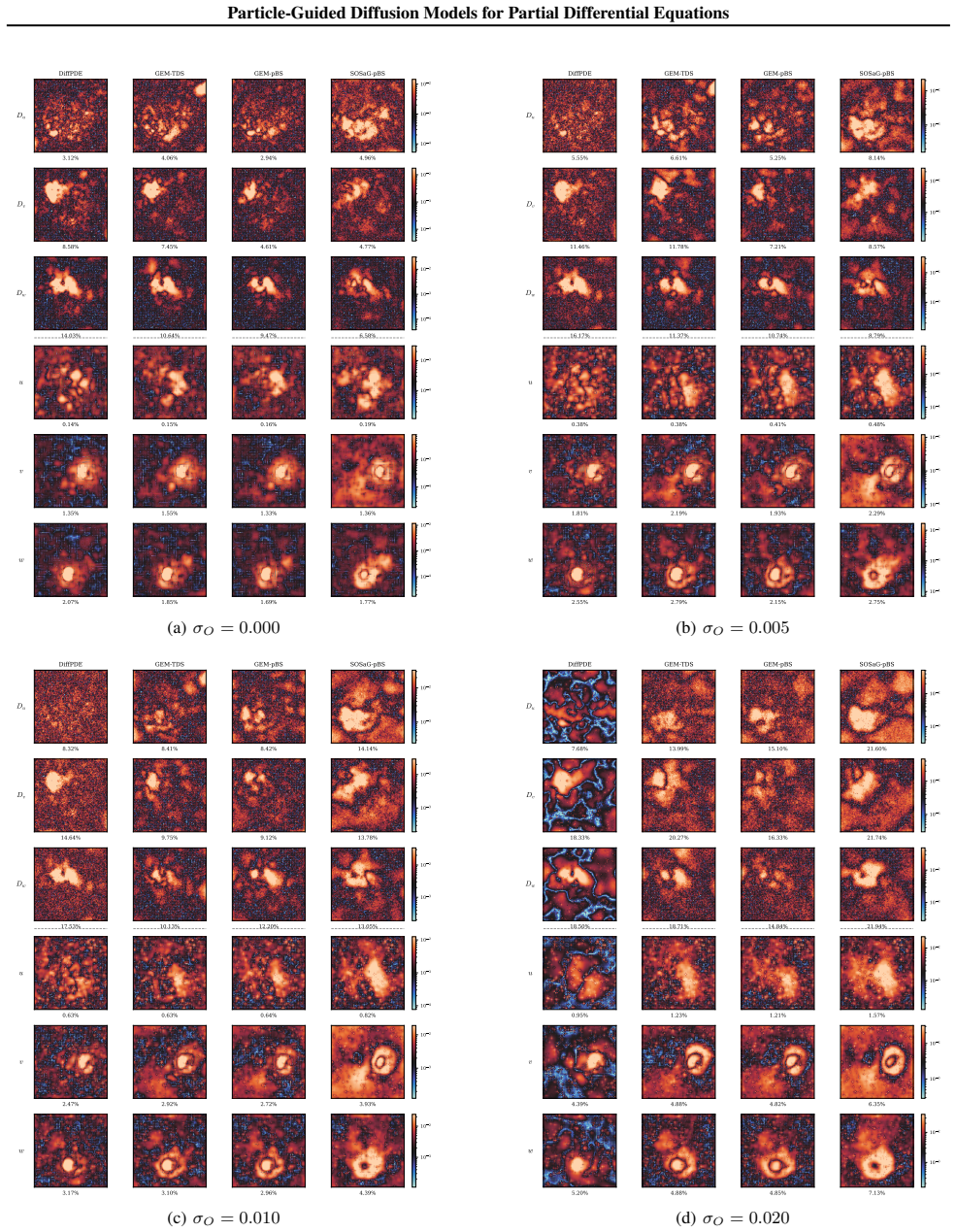
- [§3.4, Eq. (20); Appendix A.3] The load-bearing claim that pBS/SMC improves accuracy is confounded with likelihood sharpening. With ρ=1, ν0(x0)∝pθ(x0|y)p̃θ(y|x0) (Eq. 20, Appendix A.3), and pθ(x0|y) itself contains a likelihood factor via the guided proposal (Eq. 19). The effective target is therefore approximately p(x0)p̃θ(y|x0)^2; for the Gaussian/MSE likelihood (Eq. 10) this is equivalent to doubling β, γ, and ω. Thus SOSaG-pBS may simply be SOSaG with sharper likelihood. To support the abstract's causal claim, add matched controls that hold the target fixed (e.g., SOSaG with β,γ,ω doubled vs SOSaG-pBS at the original values), and report ρ=1 with equivalent precision.
- [Table 1] Table 1 does not support the blanket claim in the abstract. SOSaG-pBS is worse than DiffPDE on Poisson inverse (24.61 vs 19.88), NS bounded inverse (11.24 vs 9.34), and Helmholtz inverse (20.50 vs 19.14). Since all results are averaged over 30 runs without error bars, even the favorable differences (e.g., Darcy forward 3.96 vs 5.58) are not statistically established. Qualify the claim to the settings where pBS helps and include confidence intervals or run-level variance.
- [Tables 4–6; §6] The effect of the pBS target is not isolated. Table 6 removes the SMC resampling/propagation but only for the non-pBS variants GEM and SOSaG; the pBS rows are not compared against a non-SMC sampler targeting the same ν0. Table 4 shows that increasing ρ often lowers error (e.g., Poisson inverse 24.13→20.17) and Figure 3 shows ESS collapses as ρ grows, which is exactly the signature of likelihood tempering. The guidance weights in Table 5 are also tuned per problem. Report sensitivity to β, γ, ω, ρ, and include an ablation that separates target change from particle interaction.
- [Eq. (11); §3.1] The intermediate likelihood p̃θ(y|x_t)=p(y|Dθ(x_t,σ_t)) is used for every weight and guidance gradient, but the approximation is unvalidated; unlike DPS-style guidance in image inverse problems, here the reconstructed field is fed into a PDE residual, which is highly nonlinear. Since pBS exponentiates this quantity, a biased likelihood estimator can be amplified. Provide at least one check (e.g., Monte Carlo estimate of ∫p(y|x0)pθ(x0|x_t)dx0 on a small set) to show the approximation is not the driver of the pBS gain.
minor comments (5)
- [Algorithm 3] Line 5 uses (σ_{k-1} − σ̂_k)d_k while Eq. (18) uses (σ_{k-1}^2 − σ̂_k^2); clarify which update is actually implemented and whether this is a typo or a deliberate simplification.
- [§2.3–2.4] The continuous time t and discrete step k are used inconsistently; for example Eq. (7) is written with t while the SMC discussion uses k. Please make the discretization explicit in the main text.
- [Table 1 caption] The caption says 'error rate' for Darcy inverse but relative L2 error elsewhere; define what is measured for the Darcy inverse case and why it differs.
- [Appendix A.5] The statement that pBS 'does not trade between posterior exactness and empirical performance' is misleading: pBS is exact for an alternative target, not for Eq. (8). The wording should acknowledge this directly.
- [Reproducibility] The paper does not mention a code release or provide random-seed and hyperparameter sweep details. Given the sensitivity to Table 5 weights and ρ, these details are important for reproducibility.
Circularity Check
No significant circularity: the pBS target is an explicitly altered target, not a hidden reduction.
full rationale
The paper's derivation chain is self-contained. The SMC/FK algebra in Appendix A.3 correctly derives the pBS target ν0(x0) ∝ pθ(x0|y)p̃θ(y|x0), and the main text explicitly acknowledges that this differs from the posterior of Eq. (8) and that it 'is essentially changing the precision of the PDE residual likelihood' (Section 3.4). This is a deliberate design choice, not a claim that the pBS target is the exact posterior, so there is no self-definitional step. The empirical improvement of SOSaG-pBS over DiffPDE is a benchmark observation; the paper does not present this superiority as a formal derivation from the SMC framework. The guidance weights in Table 5 are hand-tuned per problem, but this is a hyperparameter-tuning confound, not a fitted parameter being renamed as a prediction. The paper's self-citations (Zhao 2026; Zhao et al. 2025; Kelvinius et al. 2025; etc.) appear only in related-work discussion and are not load-bearing: the pBS target is derived locally, and no uniqueness theorem or external result is imported from those citations to force the method. The closest concern to circularity is that pBS with ρ=1 approximately squares the likelihood, which could mean the reported gains come from likelihood sharpening rather than particle interaction. But the paper states this behavior openly (Section 3.4 and Appendix A.5), and the equivocation is a matter of interpretation of empirical results, not a derivation that reduces to its own inputs by construction. Under the provided rules, that is not circularity.
Axiom & Free-Parameter Ledger
free parameters (4)
- Guidance weights β, γ, ω (per experiment) =
e.g., Darcy: γ=5, β=5000, ω=100; 2SRD: γ=7, β=20, ω=2 (Table 5)
- Tempering parameter ρ =
1 in main results; 5–1000 explored in Table 4
- SMC particle count N =
4
- Diffusion steps K =
2000
axioms (5)
- domain assumption Learned denoiser Dθ(x,σ) accurately approximates the true score (EDM framework)
- domain assumption p̃θ(y|x_t)=p(y|Dθ(x_t,σ_t)) is a faithful proxy for the intractable p_t(y|x_t)
- standard math Feynman–Kac/SMC consistency for the chosen proposal/potential pair
- ad hoc to paper The altered pBS target is a better target for PDE solving than the posterior in Eq. (8)
- domain assumption FEM-generated data used as ground truth for evaluation
read the original abstract
We introduce a guided stochastic sampling method that augments sampling from diffusion models with physics-based guidance derived from partial differential equation (PDE) residuals and observational constraints, ensuring generated samples remain physically admissible. We embed this sampling procedure within a new Sequential Monte Carlo (SMC) framework, yielding a scalable generative PDE solver. Across multiple benchmark PDE systems as well as multiphysics and interacting PDE systems, our method produces solution fields with lower numerical error than existing state-of-the-art generative methods.
Figures


Forward citations
Cited by 2 Pith papers
-
Flow Learners for PDEs: Toward a Physics-to-Physics Paradigm for Scientific Computing
Flow learners parameterize transport vector fields to generate PDE trajectories through integration, offering a physics-to-physics organizing principle for learned solvers.
-
Flow Learners for PDEs: Toward a Physics-to-Physics Paradigm for Scientific Computing
Learned PDE solving should target transport over admissible futures via flow learners, not snapshot state regression.
Reference graph
Works this paper leans on
-
[1]
URL https:// doi.org/10.1007/978-1-4684-9393-1_2
doi: 10.1007/978-1-4684-9393-1 2. URL https:// doi.org/10.1007/978-1-4684-9393-1_2. Dhariwal, P. and Nichol, A. Diffusion Models Beat GANs on Image Synthesis.Advances in Neural Information Processing Systems, 34:8780–8794, 2021. Dou, Z. and Song, Y . Diffusion Posterior Sampling for Linear Inverse Problem Solving: A Filtering Perspective. InThe Twelfth In...
Pith/arXiv arXiv 2021
-
[2]
In pBS, each particle receives an incremental weight Gj−1(xj, xj−1) = ˜pθ(y|x j−1) ˜pθ(y|x j)
Fitness evaluation ← →Weighting.In an EA, each offspring is assigned a scalar fitness value. In pBS, each particle receives an incremental weight Gj−1(xj, xj−1) = ˜pθ(y|x j−1) ˜pθ(y|x j) . 17 Particle-Guided Diffusion Models for Partial Differential Equations In the deterministic (PDE) setting, the approximate likelihood ˜pθ(y|x j−1) measures how well the...
-
[3]
Huang, R., Huang, J., Yang, D., Ren, Y ., Liu, L., Li, M., Ye, Z., Liu, J., Yin, X., and Zhao, Z
URL https://openreview.net/forum? id=z0I2SbjN0R. Huang, R., Huang, J., Yang, D., Ren, Y ., Liu, L., Li, M., Ye, Z., Liu, J., Yin, X., and Zhao, Z. Make-an-Audio: Text-to-Audio Generation with Prompt-Enhanced Diffu- sion Models. InInternational Conference on Machine Learning, pp. 13916–13932. PMLR, 2023. Janati, Y ., Moufad, B., Abou El Qassime, M., Durmus...
arXiv 2023
-
[5]
URL https://openreview.net/forum? id=5EdFkEmjr3. Kondo, S. and Miura, T. Reaction-Diffusion Model as a Framework for Understanding Biological Pattern Forma- tion.Science, 329(5999):1616–1620, 2010. doi: 10.1126/ science.1179047. URL https://www.science. org/doi/abs/10.1126/science.1179047. Kong, Z., Ping, W., Huang, J., Zhao, K., and Catanzaro, B. DiffWav...
-
[9]
URL https://openreview.net/forum? id=eWKqr1zcRv. Yang, G. and Sommer, S. A Denoising Diffusion Model for Fluid Field Prediction.arXiv preprint arXiv:2301.11661, 2023. Yim, J., St ¨ark, H., Corso, G., Jing, B., Barzilay, R., and Jaakkola, T. S. Diffusion Models in Protein Structure and Docking.Wiley Interdisciplinary Reviews: Computa- tional Molecular Scie...
Pith/arXiv arXiv 2023
-
[10]
In pBS, each particle is propagated via the guided sampler x(i) j−1 ∼M j−1(· |xj) = ˜pθ(xj−1 |x j, y)
Mutation ← →Proposal.In an EA, each individual xj in the population is stochastically perturbed to produce an offspring x(i) j−1. In pBS, each particle is propagated via the guided sampler x(i) j−1 ∼M j−1(· |xj) = ˜pθ(xj−1 |x j, y). Both operations apply a stochastic perturbation to each member of the population independently, conditional on its current state
-
[12]
Selection ← →Resampling.In an EA, individuals are selected for the next generation with probability proportional to their fitness. In SMC, when the effective sample size drops below Neff, particles are resampled with probability proportional to their normalised weights. Both operations duplicate high-fitness/high-weight individuals and discard low-fitness...
arXiv 2024
-
[2020]
Shysheya, A., Diaconu, C., Bergamin, F., Perdikaris, P., Hern´andez-Lobato, J
URL https://proceedings.mlr.press/ v119/sanchez-gonzalez20a.html. Shysheya, A., Diaconu, C., Bergamin, F., Perdikaris, P., Hern´andez-Lobato, J. M., Turner, R. E., and Mathieu, E. On conditional diffusion models for PDE simula- tions. InThe Thirty-eighth Annual Conference on Neural Information Processing Systems, 2024. URL https: //openreview.net/forum?id...
2024
-
[2021]
Stevens, T
URL https://openreview.net/forum? id=PxTIG12RRHS. Stevens, T. S., Nolan, O., Robert, J.-L., and Van Sloun, R. J. Sequential Posterior Sampling with Diffusion Models. In ICASSP 2025–2025 IEEE International Conference on Acoustics, Speech and Signal Processing (ICASSP), pp. 1–5. IEEE, 2025. Strauss, W. A.Partial Differential Equations: An Introduc- tion. Jo...
2025
-
[2022]
Kelvinius, F
URL https://openreview.net/forum? id=k7FuTOWMOc7. Kelvinius, F. E., Zhao, Z., and Lindsten, F. Solving Linear- Gaussian Bayesian Inverse Problems with Decoupled Diffusion Sequential Monte Carlo. InProceedings of the 10 Particle-Guided Diffusion Models for Partial Differential Equations 42nd International Conference on Machine Learning, vol- ume 267 ofProc...
2025
-
[2023]
URL https://proceedings.mlr.press/ v202/liu23f.html. Liu, Q. and Thuerey, N. Uncertainty-Aware Surrogate Mod- els for Airfoil Flow Simulations with Denoising Diffusion Probabilistic Models.AIAA Journal, 62(8):2912–2933, 2024. Lu, L., Jin, P., and Karniadakis, G. E. DeepONet: Learning Nonlinear Operators for Identifying Differential Equa- tions Based on th...
Pith/arXiv arXiv 2024
-
[2024]
URL https://openreview.net/forum? id=nHESwXvxWK. 9 Particle-Guided Diffusion Models for Partial Differential Equations Chopin, N., Papaspiliopoulos, O., et al.An Introduction to Sequential Monte Carlo, volume 4. Springer, 2020. Chung, H., Kim, J., and Ye, J. C. Diffusion models for inverse problems, 2025. URL https://arxiv.org/ abs/2508.01975. Corenflos, ...
Pith/arXiv arXiv 2020
discussion (0)
Sign in with ORCID, Apple, or X to comment. Anyone can read and Pith papers without signing in.