Voronoi-grid-based Pareto Front Learning and Its Application to Collaborative Federated Learning

Han Yu; Mengmeng Chen; Qicheng Lao; Qiqi Liu; Tiantian He; Xiaohu Wu; Yaochu Jin; Yew-Soon Ong

REVIEW 3 major objections 5 minor 22 references

Voronoi-grid-based Pareto Front Learning and Its Application to Collaborative Federated Learning

T0 review · 3 major / 5 minor · reviewed 2026-08-07 · deepseek-v4-flash

Challenge this review Re-run · record.json Download PDF Read on arXiv ↗

Pith's one-line read Pareto-front learning now covers convex boundaries too

desk verdict Useful Voronoi sampling idea and broad experiments, but Algorithm 2's penalty sign contradicts Eq. (13), so the stated coverage mechanism is not implemented; fix that before believing the coverage claims. read the letter →

arxiv 2505.20648 v1 pith:FPEHZWWN submitted 2025-05-27 cs.LG cs.AI

Mengmeng Chen , Xiaohu Wu , Qiqi Liu , Tiantian He , Yew-Soon Ong , Yaochu Jin , Qicheng Lao , Han Yu This is my paper · ORCID

classification cs.LGcs.AI

keywords Paretofrontlearninghypernetworkmulti-objectiveoptimizationhypervolumeindicatorVoronoidiagramgeneticalgorithmfederatedbenefitgraph

verification ladder T0 review T1 audit T2 compute T3 formal

The pith

A machine-rendered reading of the paper's core claim, the machinery that carries it, and where it could break.

The reading

The paper proposes PHN-HVVS, a Pareto-front-learning method in which a hypernetwork maps preference vectors to solutions. It targets two known failures of earlier Pareto hypernetworks: poor sampling of preference rays in high-dimensional objective spaces, and solution sets that cluster in the middle of the front and miss convex boundary regions. The method partitions the preference simplex into Voronoi cells using a genetic algorithm, draws one preference vector per cell, and trains with a loss that combines hypervolume maximization with a distance penalty pulling each solution toward its assigned preference direction. The authors report that this yields fuller, higher-hypervolume Pareto fronts on toy, multi-task, and federated-learning benchmarks, and that the improved fronts translate into better benefit graphs, the directed graphs that encode how much one federated-learning participant's data helps another.

What carries the argument

The central object is a Voronoi partition of the preference hyperplane $H=\{x\in\mathbb{R}^J : \sum_j x_j=1\}$: a genetic algorithm evolves $N$ sites so that Monte Carlo sample points are split as evenly as possible across the cells, with uniformity scored by $O=1/(1+\rho)$ in Eq. (12), and one preference vector is then drawn from each cell. This provides an arbitrary number of rays in any dimension, bypassing the combinatorial uniform designs whose point counts grow like $\binom{J+k-1}{k}$. The second mechanism is the distance penalty $D(r_i,\ell_i)$ of Eq. (14), the distance from the generated loss vector to the line through its preference vector along $u=(1,\ldots,1)$; the paper argues that its gradient pushes each output toward the boundary region consistent with that preference, counteracting the weight decay that concentrates gradient-based HV maximization on intermediate solutions. The HV gradient, computed with an exact multi-sweep derivative, and the penalty make up the update rule of Algorithm 2.

What would settle it

Run PHN-HVVS on a disconnected or strongly irregular Pareto front, such as ZDT3 with separated components, and measure per-region coverage against the true front: if the solutions cluster on one component or leave boundary gaps while hypervolume stays high, the coverage claim fails. A second check is to set $\lambda=0$ in Eq. (13): if hypervolume and coverage are unchanged, the distance penalty is not what carries the result.

Watch

Extended reading notes

Core claim

At the core is the claim that uniform coverage of the preference simplex, enforced by a Voronoi partition whose cells are made equally populated by a genetic algorithm, plus the distance-based penalty of Eq. (14), is enough to make the hypernetwork's output set cover the entire Pareto front rather than only its central region. The training objective is $\min_\phi \mathbb{E}[Q(L(\Theta,x,y))] + \lambda \sum_i D(r_i,\ell_i)$ with $Q=-HV$ and $D(r_i,\ell_i)$ the Euclidean distance from the loss vector $\ell_i$ to the line through its preference point $r_i$ in direction $u=(1,\ldots,1)$; the HV term drives convergence to the true front, while the penalty spreads solutions toward boundary regions that gradient-based HV maximization tends to ignore. The paper reports that on convex fronts the solutions trace the whole true front, that its hypervolume exceeds all compared baselines on the tested tasks, and that plugging the method into three federated-learning benefit-graph pipelines improves accuracy or AUC.

Load-bearing premise

The load-bearing premise is that equal cell counts on the preference simplex, together with the line-pulling distance penalty, force the learned solution set to cover the entire Pareto front in objective space, including convex boundary regions, for any problem shape.

Editorial extensions

If this is right

The number of preference vectors becomes a free parameter in any dimension, because Voronoi sampling replaces combinatorial uniform-design constructions.
Convex Pareto fronts, where previous hypervolume-gradient methods concentrate in the middle, can be covered to the boundaries; the paper shows boundary solutions appearing on Problems 1, 5, and 7.
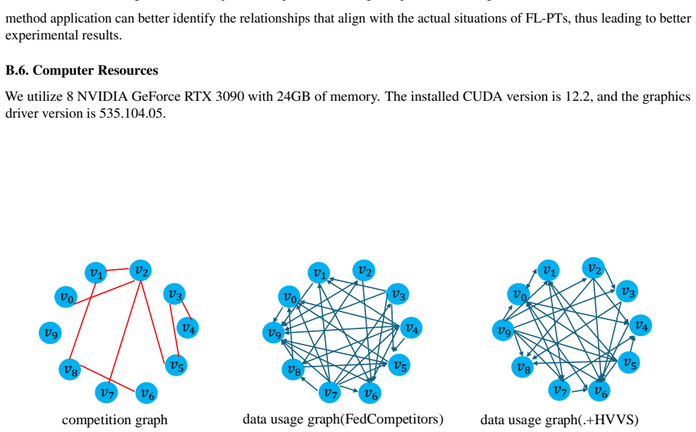
Federated-learning benefit graphs are built from more precise per-client preference vectors, and the paper reports that three benefit-graph pipelines improve on CIFAR-10 accuracy and eICU AUC.
The Voronoi grid is constructed once and reused in every training round, so per-round sampling becomes a lookup rather than a fresh partition.
The whole training objective still has a single parameter set (the hypernetwork weights $\phi$), so no per-objective scalarization tuning is introduced.

Reading between the lines

Editorial extensions of the paper, not claims the author makes directly.

The distance penalty is a geometric surrogate for coverage: it assumes the line through $r_i$ is a good target for $\ell_i$. On sharply bent or disconnected fronts the penalty could pull solutions to points on that line that are not on the front, so coverage should be checked with gap measures such as per-region occupancy or inverted generational distance rather than hypervolume alone.
Equal cell counts are enforced in preference space; the method assumes this carries over to even spacing in objective space. A stress test with a front of strongly unequal curvature, such as a flat tail plus a sharp knee, would show whether the two uniformities diverge.
A natural extension the paper does not try is to anneal the penalty weight $\lambda$ during training, starting large to seed boundary solutions and then letting hypervolume dominate; a fixed $\lambda$ may not be optimal for all front shapes.
The Voronoi sampler is decoupled from the hypernetwork, so the same partition could be reused by other decomposition-based multi-objective optimizers; the paper does not explore that transfer.

Share X Bluesky LinkedIn Reddit HN

Editorial analysis

A structured set of objections, weighed in public.

Desk editor's note, referee report, and a circularity audit.

Desk Editor's Note

read the letter

Quick take: the Voronoi sampling piece is a real improvement and the experiments are broad, but the paper has a load-bearing sign bug in its own algorithm. The stress-test note is right. Eq. (13) minimizes λ Σ D(r_i, ℓ_i), but Algorithm 2's update maximizes it. Spelled out: the update computes g = -dHV/dϕ, then g_update = g - λ dD/dϕ, then ϕ ← ϕ - η g_update. That yields ϕ + η dHV/dϕ + η λ dD/dϕ, i.e., gradient ascent on HV + λ D. So the implemented penalty increases the distance from ℓ_i to the line through r_i in direction (1,...,1), while Eq. (13) and the text say it should decrease it. The paper's coverage story rests on that penalty, so as written the described mechanism and the actual optimization are opposite. The empirical results might still be reproducible with a "maximize distance" implementation, but the paper cannot be read as testing its stated hypothesis until this is resolved.

What is genuinely new: Voronoi-based GA sampling of the preference simplex is a sensible fix for the high-dimensional ray-sampling problem, and the downstream application to federated benefit graphs is a legitimate use case. The benchmark coverage is wide and the method usually wins on HV, especially on the 2D problems. Code is public.

Soft spots beyond the sign issue: "significant" appears without a single significance test; on Jura and SARCOS the gains are about 1%, inside the 1–5% Monte Carlo error the authors themselves report for HV when J>3. The coverage argument is geometric intuition, not a derivation: no proof that the penalty, with any λ, yields complete coverage rather than clustering or misalignment. Hyperparameters λ, GA population size, generations, and M are not reported, which hurts reproducibility. The FL improvements are real but small (e.g., 82.19→82.44 on one setting), and some standard deviations overlap.

Bottom line: this deserves a serious referee, because the core idea is worth engaging with and the flaw is addressable. But the sign contradiction is exactly the kind of thing that has to be fixed before the paper can be believed, and the empirical claims need statistical backing.

Referee Report

3 major / 5 minor

Summary. The paper proposes PHN-HVVS, a Pareto-front learning method for multi-objective optimization. It uses a genetic algorithm to construct a Voronoi partition of the preference simplex, samples preference vectors from the resulting cells, and trains a hypernetwork with a loss that combines negative hypervolume (HV) with a distance penalty D(r_i, ℓ_i) intended to spread the generated solutions across the entire Pareto front, including convex boundary regions. The method is evaluated on eight toy problems, several multi-task learning datasets, and three federated-learning benefit-graph frameworks. The authors report higher HV than existing PHN variants on most benchmarks and claim significant improvements, especially on convex fronts.

Significance. If the claims were fully supported, the paper would make a useful contribution to Pareto-front learning: the Voronoi-based sampling addresses a real high-dimensional ray-sampling problem, and the proposed loss targets the known convex-front coverage failure of HV-gradient methods. The paper has strengths: code is provided, experiments cover many benchmarks, five independent runs are reported, and Appendix B.4 includes an ablation of sampling strategies. However, the central algorithmic claim is undermined by a sign inconsistency between the stated objective and the reported update rule, and the empirical support for the word "significantly" is weak in the higher-dimensional cases where HV is estimated by Monte Carlo. As written, the mechanism claimed to produce coverage is not the mechanism actually described by the pseudocode, so the validity of the central claim is not established.

major comments (3)

[Section 4.2, Eq. (13), Algorithm 2] The update rule in Algorithm 2 does not minimize the loss defined in Eq. (13). Eq. (13) is min_φ E[-HV(L)] + λ Σ_i D(r_i, ℓ_i); standard gradient descent on this objective gives φ ← φ + η ∂HV/∂φ - η λ ∂(Σ D)/∂φ. Algorithm 2 instead computes g = -∂HV/∂φ (line 8), then g_update = g - λ ∂(Σ D)/∂φ (line 9), and φ ← φ - η g_update (line 10), which evaluates to φ + η ∂HV/∂φ + η λ ∂(Σ D)/∂φ. The penalty term therefore has the opposite sign: the algorithm maximizes Σ_i D(r_i, ℓ_i), which is the opposite of the coverage mechanism described in the text. The reported experimental results cannot be attributed to the Eq. (13) objective as written; the authors must correct either the pseudocode or the objective and verify whether the claimed coverage improvement survives.
[Section 5, Tables 1 and 8, Appendix B.4] The paper uses the word "significantly" without any significance tests, and several reported differences are within the admitted Monte Carlo error. The text states that for J > 3 the HV computation has an error of 1% to 5%; the Jura and SARCOS improvements in Table 1 are about 0.013 and 0.010 (about 1.4% and 1.1% relative), and the five-run standard deviations overlap with the PHN-HVI baseline (Jura: 0.935 ± 0.013 vs 0.922 ± 0.044; SARCOS: 0.939 ± 0.026 vs 0.929 ± 0.031). The same pattern appears for several multi-task datasets. I request either paired significance tests across runs, an explicit accounting of the Monte Carlo HV error, or more cautious wording. The abstract's "outperforms the baselines significantly" is not justified by the current evidence.
[Section 4.1.2 and 4.2, Eqs. (11)-(14)] The paper asserts, but does not demonstrate, that equal-count Voronoi cells in preference space and the distance penalty D(r_i, ℓ_i) yield complete coverage of the Pareto front, especially on convex boundary regions. Eq. (14) defines D as the perpendicular distance from ℓ_i to the line through r_i with direction u = (1, ..., 1); no derivation or counterexample analysis is given to show that minimizing this term spreads solutions across the whole front rather than, for example, aligning them along a different curve or clustering at endpoints. The statement in Section 4.2 that the penalty "ensures that the resulting distribution covers the entire Pareto front, regardless of its shape" is therefore not supported by the presented analysis. I recommend adding a formal or carefully tested geometric justification and an ablation over the penalty weight λ.

minor comments (5)

[Figure 1] The caption or figure contains the Chinese placeholder "在此处键入公式。" which should be removed or replaced with the intended mathematical expression.
[Algorithm 2] Line 1 reads "while not converged do do"; the duplicated "do" is a typo.
[Section 4.2, Eq. (14)] The direction vector is denoted u in Eq. (14) and in the notation table, but v in the surrounding text and in Figure 4; the notation should be unified.
[Section 5] The sentence describing the HV Monte Carlo error says the error is 1% to 5% when J > 3; since Jura (J=4) and SARCOS (J=7) fall in this regime, please clarify exactly which reported numbers are affected and how the Monte Carlo error was estimated for the reported means.
[Table 2] The column header "CE .+HVVS" is unclear; the baseline "CE" is not introduced in the text and should be defined or renamed for readability.

Circularity Check

0 steps flagged · score 0.0 of 10

No significant circularity: the Voronoi sampling, HV-plus-distance loss, and experimental comparisons are self-contained and externally benchmarked; self-citations are application targets, not load-bearing evidence.

full rationale

The paper's derivation chain is self-contained rather than circular. The Voronoi sampling procedure (Algorithm 1) is defined from external building blocks (Voronoi diagrams, GA, KD-trees), and its uniformity objective in Eq. (12) is a stated design goal, not a consequence of the coverage result it is used to support. The proposed loss in Eq. (13) combines a hypervolume gradient term, taken from published work (Wang et al. 2017; Emmerich and Deutz 2014), with a newly defined distance penalty D(r_i, l_i) in Eq. (14); no fitted constant or prior result of the present authors is used to define the target coverage or HV claims. The experimental validation is conducted against external benchmarks (DTLZ2/4, ZDT1/2, VLMOP1/2, MultiMNIST, CIFAR-10, eICU) and published baselines, and the FL experiments apply PHN-HVVS inside prior frameworks such as FedCompetitors and FedEgoists. Those frameworks include the authors' own Chen et al. (2024) paper, but the citations are used as application contexts being improved, not as evidence for the Voronoi or penalty mechanisms, so they are not load-bearing. No step in the paper reduces by construction to its inputs, and no fitted parameter is renamed as a prediction. The reviewer-noted sign inconsistency between Eq. (13) and Algorithm 2 is a potential correctness or implementation-consistency issue, but it is not a form of definitional circularity and therefore does not affect the circularity score.

Assumptions & free parameters 3 free parameters · 4 assumptions · 1 invented entities

The central claim leans on four heuristic premises: the Voronoi cell-uniformity surrogate, the geometric distance-penalty surrogate, the accuracy of Monte Carlo HV estimates in high dimensions, and the benefit-graph interpretation from prior FL work. The objective in Eq. (13) contains one unreported scalar weight λ, and the Voronoi partition depends on several unreported GA parameters. No physically invented entity is needed; the Voronoi distribution is an algorithmic innovation with a direct empirical comparison.

free parameters (3)

Lambda (penalty weight in Eq. 13) = Not reported
Balances the hypervolume gradient against the distance penalty; no sensitivity analysis is given, so the reported results may depend on a tuned compromise.
GA population size, generation count, and Monte Carlo point count M = Not reported; mutation std is 0.05 and M=100000 appears in Figure 3
These parameters control the uniformity of the Voronoi partition; no ablation shows how sensitive the final front is to them.
HV reference point R = Dataset-dependent: (2,2), (1,...,1), or (3,...,3)
Adopted from Hoang et al. 2023 and shared by all baselines; it is a choice that affects absolute HV values and the size of the observed gaps.

assumptions (4)

ad hoc to paper A Voronoi partition of the preference simplex that equalizes the number of Monte Carlo points per cell (Eq. 11-12) gives a sampling distribution that covers the whole Pareto front, including convex boundary regions.
Invoked in Section 4.1.2 and Appendix A.3; no theorem connects cell-count uniformity in preference space to objective-space Pareto front coverage.
ad hoc to paper Minimizing the perpendicular distance D(ri, ℓi) from each output solution to the line through its preference ray with direction u=(1,...,1), combined with HV maximization, spreads the front and preserves Pareto optimality.
Section 4.2, Eq. (14) and the paragraph following it assert the coverage effect; the paper does not derive this or analyze failure cases.
domain assumption The Monte Carlo hypervolume estimate for J>3 has 1-5% error and is accurate enough to rank the compared methods.
The authors state this error themselves in Section 5 and Appendix B.3; several claimed improvements, Jura and SARCOS, are about 1%, so this assumption is load-bearing for those comparisons.
domain assumption The benefit-graph interpretation, where the preference vector that maximizes a client's validation performance estimates the contribution weights of other clients, is valid.
Carried over from Cui et al. 2022, Tan et al. 2024, and Chen et al. 2024 via Eq. (24); used to translate better Pareto front coverage into federated learning gains.

invented entities (1)

Voronoi distribution over the preference simplex independent evidence
purpose: Sampling distribution used by PHN-HVVS to draw one preference vector per Voronoi cell during training of the hypernetwork.
Introduced in Section 4.1.2 and empirically compared with random, Latin hypercube, polar, Dirichlet, and K-means sampling in Table 9, giving it a falsifiable handle beyond the paper's own objective. It is an algorithmic device, not a physically postulated entity.

how reviews work

0 comments

Cite this review

Pith. "Pith review of Voronoi-grid-based Pareto Front Learning and Its Application to Collaborative Federated Learning." pith.science (2026). https://pith.science/paper/FPEHZWWN

@misc{pith2026250520648,
  author       = {Pith},
  title        = {Pith review of: Voronoi-grid-based Pareto Front Learning and Its Application to Collaborative Federated Learning},
  year         = {2026},
  howpublished = {\url{https://pith.science/paper/FPEHZWWN}},
  note         = {Machine review of arXiv:2505.20648}
}

read the original abstract

Multi-objective optimization (MOO) exists extensively in machine learning, and aims to find a set of Pareto-optimal solutions, called the Pareto front, e.g., it is fundamental for multiple avenues of research in federated learning (FL). Pareto-Front Learning (PFL) is a powerful method implemented using Hypernetworks (PHNs) to approximate the Pareto front. This method enables the acquisition of a mapping function from a given preference vector to the solutions on the Pareto front. However, most existing PFL approaches still face two challenges: (a) sampling rays in high-dimensional spaces; (b) failing to cover the entire Pareto Front which has a convex shape. Here, we introduce a novel PFL framework, called as PHN-HVVS, which decomposes the design space into Voronoi grids and deploys a genetic algorithm (GA) for Voronoi grid partitioning within high-dimensional space. We put forward a new loss function, which effectively contributes to more extensive coverage of the resultant Pareto front and maximizes the HV Indicator. Experimental results on multiple MOO machine learning tasks demonstrate that PHN-HVVS outperforms the baselines significantly in generating Pareto front. Also, we illustrate that PHN-HVVS advances the methodologies of several recent problems in the FL field. The code is available at https://github.com/buptcmm/phnhvvs}{https://github.com/buptcmm/phnhvvs.

Figures

Figures reproduced from arXiv: 2505.20648 by the authors.

**Figure 1.** Multi-Sample-Hypernetwork framework 3. Preliminary The goal of Multi-task learning is to find θ ∗ ∈ Θ to optimize J loss functions: θ ∗ = arg min θ E(x,y)∼pD ℓ(y, f(x; θ)) (1) where ℓ(y, f(x; θ)) = {ℓ1(y, f(x; θ)), . . . , ℓJ (y, f(x; θ))}, pD denotes the data distribution, ℓj : Y ×Y → R>0 denotes the j-th loss function and f(x; θ) : X × ϑ → Y denotes the neural network with θ. PFL extends this framework to learn th… view at source ↗

**Figure 2.** (a) depicts the HV of the two-objective optimization problem, and [PITH_FULL_IMAGE:figures/full_fig_p003_2.png] view at source ↗

**Figure 3.** Voronoi Diagram with J = 3, N = 16, M = 100000 4.2. PHN-HVVS The Voronoi Sampling method enables sampling rays across the entire H. Building on this, we propose a new objective function to better explore the solution space and achieve a complete Pareto front. Pareto HyperNetworks with HV maximization via Voronoi Sampling (PHN-HVVS) is designed to solve the following objective: min ϕ E r∼pSJ (x,y)∼pD Q(L(Θ, x, y)) + … view at source ↗

Figures from the paper (14 more)

**Figure 4.** Figure 4: depicts D(r i , ℓi ) in 2D space. The combination of HV and the penalty term optimizes both the quality and diversity of the Pareto front. If the HV of a set of solutions reaches its maximum, then these solutions are on the Pareto front (Fleischer, 2003). The HV term i…

**Figure 5.** Figure 5: Results comparison on different Multi-Task Datasets [PITH_FULL_IMAGE:figures/full_fig_p008_5.png]

**Figure 6.** Figure 6: Pathological distribution Benefit Graph sampling distribution. Voronoi partition method ensures effective exploration of the global PF. As shown in [PITH_FULL_IMAGE:figures/full_fig_p017_6.png]

**Figure 7.** Figure 7: Dirichlet distribution Benefit Graph 𝑣1 𝑣2 𝑣3 𝑣4 𝑣5 𝑣7 𝑣6 𝑣8 𝑣0 𝑣9 𝑣1 𝑣2 𝑣3 𝑣4 𝑣5 𝑣7 𝑣6 𝑣8 𝑣0 𝑣9 𝑣1 𝑣2 𝑣3 𝑣4 𝑣5 𝑣7 𝑣6 𝑣8 𝑣0 𝑣9 𝑣1 𝑣2 𝑣3 𝑣4 𝑣5 𝑣7 𝑣6 𝑣8 𝑣0 𝑣9 𝑣1 𝑣2 𝑣3 𝑣4 𝑣5 𝑣7 𝑣6 𝑣8 𝑣0 𝑣9 𝑣1 𝑣2 𝑣3 𝑣4 𝑣5 𝑣7 𝑣6 𝑣8 𝑣0 𝑣9 competition graph data usage graph(FedCompetitors) d…

**Figure 8.** Figure 8: The Competition Graph and Data Usage Graph under Pathological distribution method application can better identify the relationships that align with the actual situations of FL-PTs, thus leading to better experimental results. B.6. Computer Resources We utilize 8 NVIDIA…

**Figure 9.** Figure 9: The Competition Graph and Data Usage Graph under Dirichlet distribution 18 [PITH_FULL_IMAGE:figures/full_fig_p018_9.png]

**Figure 10.** Figure 10: Results comparison on Problem1 0.0 0.2 0.4 0.6 0.8 0.0 0.2 0.4 0.6 0.8 PHN-HVVS 0.0 0.2 0.4 0.6 0.8 0.0 0.2 0.4 0.6 0.8 PHN-HVI 0.0 0.2 0.4 0.6 0.8 0.0 0.2 0.4 0.6 0.8 PHN-EPO 0.0 0.2 0.4 0.6 0.8 0.0 0.2 0.4 0.6 0.8 PHN-LS 0.0 0.2 0.4 0.6 0.8 0.0 0.2 0.4 0.6 0.8 COSMO…

**Figure 11.** Figure 11: Results comparison on Problem2 0.0 0.2 0.4 0.6 0.8 1.0 0.0 0.2 0.4 0.6 0.8 1.0 0.0 0.2 0.4 0.6 0.8 1.0 PHN-HVVS 0.0 0.2 0.4 0.6 0.8 1.0 0.0 0.2 0.4 0.6 0.8 1.0 0.0 0.2 0.4 0.6 0.8 1.0 PHN-HVI 0.0 0.2 0.4 0.6 0.8 1.0 0.0 0.2 0.4 0.6 0.8 1.0 0.0 0.2 0.4 0.6 0.8 1.0 PHN-…

**Figure 12.** Figure 12: Results comparison on Problem3 0.0 0.2 0.4 0.6 0.8 1.0 0.0 0.2 0.4 0.6 0.8 1.0 0.0 0.2 0.4 0.6 0.8 1.0 PHN-HVVS 0.0 0.2 0.4 0.6 0.8 1.0 0.0 0.2 0.4 0.6 0.8 1.0 0.0 0.2 0.4 0.6 0.8 1.0 PHN-HVI 0.0 0.2 0.4 0.6 0.8 1.0 0.0 0.2 0.4 0.6 0.8 1.0 0.0 0.2 0.4 0.6 0.8 1.0 PHN-…

**Figure 13.** Figure 13: Results comparison on Problem4 19 [PITH_FULL_IMAGE:figures/full_fig_p019_13.png]

**Figure 14.** Figure 14: Results comparison on Problem5 0.0 0.2 0.4 0.6 0.8 1.0 0.0 0.2 0.4 0.6 0.8 1.0 PHN-HVVS 0.0 0.2 0.4 0.6 0.8 1.0 0.0 0.2 0.4 0.6 0.8 1.0 PHN-HVI 0.0 0.2 0.4 0.6 0.8 1.0 0.0 0.2 0.4 0.6 0.8 1.0 PHN-EPO 0.0 0.2 0.4 0.6 0.8 1.0 0.0 0.2 0.4 0.6 0.8 1.0 PHN-LS 0.0 0.2 0.4 0…

**Figure 15.** Figure 15: Results comparison on Problem6 0.0 0.2 0.4 0.6 0.8 1.0 0.0 0.2 0.4 0.6 0.8 1.0 PHN-HVVS 0.0 0.2 0.4 0.6 0.8 1.0 0.0 0.2 0.4 0.6 0.8 1.0 PHN-HVI 0.0 0.2 0.4 0.6 0.8 1.0 0.0 0.2 0.4 0.6 0.8 1.0 PHN-EPO 0.0 0.2 0.4 0.6 0.8 1.0 0.0 0.2 0.4 0.6 0.8 1.0 PHN-LS 0.0 0.2 0.4 0…

**Figure 16.** Figure 16: Results comparison on Problem7 0.0 0.2 0.4 0.6 0.8 1.0 0.0 0.2 0.4 0.6 0.8 1.0 PHN-HVVS 0.0 0.2 0.4 0.6 0.8 1.0 0.0 0.2 0.4 0.6 0.8 1.0 PHN-HVI 0.0 0.2 0.4 0.6 0.8 1.0 0.0 0.2 0.4 0.6 0.8 1.0 PHN-EPO 0.0 0.2 0.4 0.6 0.8 1.0 0.0 0.2 0.4 0.6 0.8 1.0 PHN-LS 0.0 0.2 0.4 0…

**Figure 17.** Figure 17: Results comparison on Problem8 20 [PITH_FULL_IMAGE:figures/full_fig_p020_17.png]

Discussion (0). Continue with ORCID to comment.

Reference graph

Works this paper leans on

22 extracted references · 16 canonical work pages

[9]

K-means V oronoi Jura 0.928 0.922 0.928 0.923 0.925 0.935 SARCOS 0.884 0.883 0.881 0.888 0.877 0.949 B.5

Comparison of different sampling techniques on Jura and SARCOS Random Latin Polar Dir. K-means V oronoi Jura 0.928 0.922 0.928 0.923 0.925 0.935 SARCOS 0.884 0.883 0.881 0.888 0.877 0.949 B.5. The details of the federated learning experiment For the CIFAR-10 dataset, the hypernetwork leverages a 2-layer hidden MLP to generate the parameters of the target ...

work page 2024
[12]

and Grabocka, J

Ruchte, M. and Grabocka, J. Scalable pareto front ap- proximation for deep multi-objective learning. In 2021 IEEE international conference on data mining (ICDM), pp. 1306–1311. IEEE,

work page 2021
[13]

Van Veldhuizen, D. A. and Lamont, G. B. Multiobjective evolutionary algorithm test suites. In Proceedings of the 1999 ACM symposium on Applied computing, pp. 351– 357,

work page 1999
[15]

Mlae: Masked lora experts for parameter-efficient fine-tuning

Wang, J., Yang, G., Chen, W., Yi, H., Wu, X., and Lao, Q. Mlae: Masked lora experts for parameter-efficient fine-tuning. arXiv preprint arXiv:2405.18897,

arXiv
[16]

doi: 10.1109/TBDATA.2022. 3186991. Wu, X., Liu, Y ., Tang, X., Cai, W., Bai, F., Khonstantine, G., and Zhao, G. Multi-agent pickup and delivery with task deadlines. In IEEE/WIC/ACM International Conference on Web Intelligence and Intelligent Agent Technology, pp. 360–367,

work page doi:10.1109/tbdata.2022 2022
[17]

Fashion-mnist: a novel image dataset for benchmarking machine learning algorithms

Xiao, H., Rasul, K., and V ollgraf, R. Fashion-mnist: a novel image dataset for benchmarking machine learning algorithms. arXiv preprint arXiv:1708.07747,

arXiv
[19]

The hypervolume indicator revisited: On the design of pareto-compliant in- dicators via weighted integration

12 Voronoi-grid-based Pareto Front Learning Zitzler, E., Brockhoff, D., and Thiele, L. The hypervolume indicator revisited: On the design of pareto-compliant in- dicators via weighted integration. In Evolutionary Multi- Criterion Optimization: 4th International Conference, EMO 2007, Matsushima, Japan, March 5-8,

work page 2007
[21]

the friend of my enemy is my enemy

on the provided multi-objective solutions to create multiple Pareto fronts. Next, a dynamic reference point is calculated by scaling the maximum values of the objectives with a factor of 1.1. The dynamic reference point is updated to ensure that it remains outside the current solution space. Once the fronts are identified and the reference point is adjust...

work page 2022

Show all 22 references

[1997]

Aspect-based sentiment analysis of drug reviews applying cross-domain and cross-data learning

Gr¨aßer, F., Kallumadi, S., Malberg, H., and Zaunseder, S. Aspect-based sentiment analysis of drug reviews applying cross-domain and cross-data learning. In Proceedings of the 2018 international conference on digital health, pp. 121–125,

2018
[1998]

Benchmarking data heterogeneity evaluation approaches for personalized federated learning

Li, Z., Wu, X., Tang, X., He, T., Ong, Y .-S., Chen, M., Liu, Q., Lao, Q., and Yu, H. Benchmarking data heterogeneity evaluation approaches for personalized federated learning. In Yu, H., Li, X., Xu, Z., Goebel, R., and King, I. (eds.), Federated Learning in the Age of Foundat...

2024
[2000]

Wang, H., Deutz, A., B ¨ack, T., and Emmerich, M

Ac- cessed: 2023-03-09. Wang, H., Deutz, A., B ¨ack, T., and Emmerich, M. Hy- pervolume indicator gradient ascent multi-objective opti- mization. In Evolutionary Multi-Criterion Optimization: 9th International Conference, EMO 2017, M¨unster, Ger- many, March 19-22, 2017, Proce...

2023
[2002]

M., Grewal, M., Dankers, F

Deist, T. M., Grewal, M., Dankers, F. J., Alderliesten, T., and Bosman, P. A. Multi-objective learning to predict pareto fronts using hypervolume maximization. arXiv preprint arXiv:2102.04523,

arXiv
[2004]

Self-evolutionary optimization for pareto front learning

Chang, S., Yoo, K., Jang, J., and Kwak, N. Self-evolutionary optimization for pareto front learning. arXiv preprint arXiv:2110.03461,

arXiv
[2007]

Theoretical Analysis

13 Voronoi-grid-based Pareto Front Learning A. Theoretical Analysis. A.1. The Time Complexity of Algorithm 1 Initializing the population involves assigning values to an array of size N × J. Since there are num species species in total, the time complexity is O(num species × N ...

2023
[2009]

Crafting papers on machine learning

Langley, P. Crafting papers on machine learning. In Langley, P. (ed.),Proceedings of the 17th International Conference on Machine Learning (ICML 2000), pp. 1207–1216, Stan- ford, CA,

2000
[2016]

and Impedovo, D

11 Voronoi-grid-based Pareto Front Learning Pirlo, G. and Impedovo, D. V oronoi-based zoning design by multi-objective genetic optimization. In 2012 10th IAPR International Workshop on Document Analysis Systems, pp. 220–224. IEEE,

2012
[2017]

Learn- ing the pareto front with hypernetworks

Navon, A., Shamsian, A., Chechik, G., and Fetaya, E. Learn- ing the pareto front with hypernetworks. arXiv preprint arXiv:2010.04104,

2010 arXiv
[2018]

Enhancing causal discovery in federated settings with limited local samples

Guo, X., Yi, L., Wu, X., Yu, K., and Wang, G. Enhancing causal discovery in federated settings with limited local samples. In Yu, H., Li, X., Xu, Z., Goebel, R., and King, I. (eds.), Federated Learning in the Age of Foundation Models - FL 2024 International Workshops, pp. 164–...

2024
[2019]

V oronoi- based estimation of distribution algorithm for multi- objective optimization

Okabe, T., Jin, Y ., Sendoff, B., and Olhofer, M. V oronoi- based estimation of distribution algorithm for multi- objective optimization. In Proceedings of the 2004 Congress on Evolutionary Computation (IEEE Cat. No. 04TH8753), volume 2, pp. 1594–1601. IEEE,

2004
[2021]

doi: 10.1561/2200000083

ISSN 1935-8237. doi: 10.1561/2200000083. Krizhevsky, A., Hinton, G., et al. Learning multiple layers of features from tiny images

1935 doi
[2023]

Personalized feder- ated learning via learning dynamic graphs

Zhou, Z., Gao, G., Wu, X., and Lyu, Y . Personalized feder- ated learning via learning dynamic graphs. arXiv preprint arXiv:2503.05474,

arXiv
[2024]

Exploiting shared representations for personalized feder- ated learning

Collins, L., Hassani, H., Mokhtari, A., and Shakkottai, S. Exploiting shared representations for personalized feder- ated learning. In International conference on machine learning, pp. 2089–2099. PMLR,

Pith tools

Reviewed August 7, 2026 · model on record in the stance chip above.

[1] [9]

K-means V oronoi Jura 0.928 0.922 0.928 0.923 0.925 0.935 SARCOS 0.884 0.883 0.881 0.888 0.877 0.949 B.5

Comparison of different sampling techniques on Jura and SARCOS Random Latin Polar Dir. K-means V oronoi Jura 0.928 0.922 0.928 0.923 0.925 0.935 SARCOS 0.884 0.883 0.881 0.888 0.877 0.949 B.5. The details of the federated learning experiment For the CIFAR-10 dataset, the hypernetwork leverages a 2-layer hidden MLP to generate the parameters of the target ...

work page 2024

[2] [12]

and Grabocka, J

Ruchte, M. and Grabocka, J. Scalable pareto front ap- proximation for deep multi-objective learning. In 2021 IEEE international conference on data mining (ICDM), pp. 1306–1311. IEEE,

work page 2021

[3] [13]

Van Veldhuizen, D. A. and Lamont, G. B. Multiobjective evolutionary algorithm test suites. In Proceedings of the 1999 ACM symposium on Applied computing, pp. 351– 357,

work page 1999

[4] [15]

Mlae: Masked lora experts for parameter-efficient fine-tuning

Wang, J., Yang, G., Chen, W., Yi, H., Wu, X., and Lao, Q. Mlae: Masked lora experts for parameter-efficient fine-tuning. arXiv preprint arXiv:2405.18897,

arXiv

[5] [16]

doi: 10.1109/TBDATA.2022. 3186991. Wu, X., Liu, Y ., Tang, X., Cai, W., Bai, F., Khonstantine, G., and Zhao, G. Multi-agent pickup and delivery with task deadlines. In IEEE/WIC/ACM International Conference on Web Intelligence and Intelligent Agent Technology, pp. 360–367,

work page doi:10.1109/tbdata.2022 2022

[6] [17]

Fashion-mnist: a novel image dataset for benchmarking machine learning algorithms

Xiao, H., Rasul, K., and V ollgraf, R. Fashion-mnist: a novel image dataset for benchmarking machine learning algorithms. arXiv preprint arXiv:1708.07747,

arXiv

[7] [19]

The hypervolume indicator revisited: On the design of pareto-compliant in- dicators via weighted integration

12 Voronoi-grid-based Pareto Front Learning Zitzler, E., Brockhoff, D., and Thiele, L. The hypervolume indicator revisited: On the design of pareto-compliant in- dicators via weighted integration. In Evolutionary Multi- Criterion Optimization: 4th International Conference, EMO 2007, Matsushima, Japan, March 5-8,

work page 2007

[8] [21]

the friend of my enemy is my enemy

on the provided multi-objective solutions to create multiple Pareto fronts. Next, a dynamic reference point is calculated by scaling the maximum values of the objectives with a factor of 1.1. The dynamic reference point is updated to ensure that it remains outside the current solution space. Once the fronts are identified and the reference point is adjust...

work page 2022