Transformer-Based Spatial-Temporal Counterfactual Outcomes Estimation

Haoang Chi; He Li; Liyang Xu; Mingyu Liu; Wanrong Huang; Wenjing Yang

REVIEW 3 major objections 5 minor 47 references

Transformer-Based Spatial-Temporal Counterfactual Outcomes Estimation

T0 review · 3 major / 5 minor · reviewed 2026-08-06 · deepseek-v4-flash

Challenge this review Re-run · record.json Download PDF Read on arXiv ↗

Pith's one-line read A Transformer-based IPW estimator is claimed to give consistent, asymptotically normal counterfactual outcomes for spatial-temporal point patterns.

desk verdict A well-written deep-learning IPW estimator for spatio-temporal counterfactual outcomes whose headline theory does not match the implemented method: the count-based propensity score is not the full-pattern score analyzed, and the martingale proof has a measurability gap. read the letter →

arxiv 2506.21154 v1 pith:G3ZXYQJ5 submitted 2025-06-26 stat.ME cs.AIcs.LG

He Li , Haoang Chi , Mingyu Liu , Wanrong Huang , Liyang Xu , Wenjing Yang This is my paper

classification stat.MEcs.AIcs.LG MSC 62D2062M3062G20

keywords spatial-temporalcausalinferencecounterfactualoutcomeestimationinverseprobabilityweightingpropensityscorespatialpointprocessTransformerasymptoticnormalityconflictandforestloss

verification ladder T0 review T1 audit T2 compute T3 formal

The pith

A machine-rendered reading of the paper's core claim, the machinery that carries it, and where it could break.

The reading

This paper tries to establish that counterfactual outcome estimation for spatial-temporal point-pattern data can be carried out by a deep inverse-probability-weighting estimator whose two learned pieces are a CNN-based propensity score and a Transformer-based outcome intensity. If correct, this would replace hand-specified kernel methods and scalar treatment summaries with a single deep model that answers what-if questions about treatment strategies that may never appear in the observed data. The authors claim the estimator is consistent and asymptotically normal under unconfoundedness, overlap, and Poisson-process assumptions, and that simulations show lower relative error than four baselines. A real-data application estimates the effect of conflict on forest loss in Colombia and concludes that longer and more intense conflicts cause more forest loss.

What carries the argument

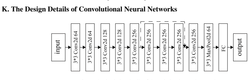
The load-bearing object is the IPW estimator $\hat{N}_t^\omega(F_H)=\int_\omega \hat{Y}_t(F_H,s)\,ds$ with $\hat{Y}_t(F_H,s)=\prod_{j=t-M+1}^t \frac{p_{h_j}(z_j)}{e_j(z_j)}\,\lambda_{Y_t^{ob}(z_{\le t})}(s)$, where the product reweights observed outcome intensity by the ratio of counterfactual to observed treatment probabilities. Its two supporting mechanisms are the dimension-reduction map $R(Z_t)=|\{s:Z_t(s)=1\}|$, which turns a high-dimensional treatment pattern into a Poisson count for both propensity and counterfactual probabilities, and a Transformer network that estimates the outcome intensity by maximizing the Poisson point-process likelihood with a KL regularization term. The proof of Proposition 3 decomposes estimation error into a martingale difference series, which obeys a central limit theorem, and a smoothing error, which is assumed to vanish faster than $1/\sqrt{T}$.

What would settle it

Simulate outcomes whose intensity at each location depends on distances to treated locations, vary only the spatial arrangement of treated points while fixing their total number, and check whether the count-based estimator's bias moves with that arrangement.

Watch

Extended reading notes

Core claim

On the paper's own terms, the central discovery is that the spatial-temporal potential-outcomes framework can be realized by an inverse-probability-weighting estimator in which both unknown ingredients are learned: the propensity score is obtained from a CNN together with a Poisson count reduction of the high-dimensional treatment pattern, and the outcome intensity is obtained from a Transformer-based neural point process. Under unconfoundedness, overlap, boundedness, and Poisson assumptions, the paper proves that the mean counterfactual outcome estimator is consistent and asymptotically normal by splitting the error into a treatment-assignment martingale difference term and a neural-network smoothing term that is assumed to vanish. Simulation experiments are offered as evidence that this estimator has lower relative error than MSMs, RMSNs, Causal Forest, and linear regression baselines, and a real-data experiment estimates the causal effect of conflict on forest loss in Colombia.

Load-bearing premise

The load-bearing premise is that replacing a whole spatial treatment pattern by the single count of treated locations preserves everything the counterfactual estimator needs, even though the consistency proof concerns the full-pattern propensity score rather than the count-based score actually implemented.

Editorial extensions

If this is right

Because the estimator is asymptotically normal, confidence intervals can in principle be attached to counterfactual outcome estimates under the stated assumptions.
The time-varying intervention distributions allow counterfactual questions about treatment strategies that never appear in the observed data, including strategies with multi-period carryover effects.
The CNN propensity module makes high-dimensional point-pattern treatments tractable, so spatial-temporal counterfactual estimation no longer relies on scalar summaries or hand-specified kernels.
The real-data conclusion implies that longer and more intense conflict in Colombia leads to more forest loss, matching the direction of prior findings in the environmental-conflict literature.

Reading between the lines

Editorial extensions of the paper, not claims the author makes directly.

We infer that the framework is most vulnerable when outcomes depend on the spatial layout of treated locations rather than only on their number; a natural test is to compare the count-based weights against full-pattern weights on small spatial grids where full-pattern propensity scores are computable.
We infer that replacing the Poisson count summary with richer spatial summaries, such as nearest-neighbor distances or point-pattern embeddings, would let the same IPW-plus-Transformer architecture extend to repulsive or clustered treatment processes.
We infer that the Colombia application could be stress-tested by varying the intervention horizon M and the intensity constant c across years or subregions to see whether the monotone forest-loss response is stable rather than an artifact of the chosen counterfactual strategy.

Share X Bluesky LinkedIn Reddit HN

Editorial analysis

A structured set of objections, weighed in public.

Desk editor's note, referee report, and a circularity audit.

Desk Editor's Note

read the letter

You should know: this is a deep-learning IPW estimator for spatio-temporal counterfactual outcomes, combining CNN-based propensity scores with a Transformer intensity model. The architecture is new and the real-data application is interesting, but the central statistical claims do not hold up as written.

What is genuinely new: the specific combination of count-reduced propensity scores with Transformer-based intensity estimation for IPW in spatio-temporal point processes. The paper is clearly organized, releases code, and extends the intervention setup to allow time-varying F_ht (a small but real generalization over Papadogeorgou et al.). The synthetic ablation relaxing the Poisson assumption is a nice empirical touch.

Three load-bearing problems. First, the theory (Proposition 3) and its proof work with full-pattern propensity scores e_j(z_j), but Section 4.6.1 replaces treatment patterns by their counts R(Z_t) and redefines both propensity and counterfactual probabilities in terms of those counts. The paper asserts this reduction "preserves the information in the treatments," but the paper's own outcome intensity (Eq. 18) depends on distances to treated locations, not just the number of treated points. So the estimator actually run in experiments need not be the estimator whose consistency is proven. Second, in the proof of Lemma 1, E1t contains N_ω(Y_t), which is not measurable with respect to the claimed filtration H_{≤t-M+1}; the martingale difference condition fails. Third, Assumptions 3(c)-(d) essentially assume the integrated neural-network bias is o(1/√T), i.e., they assume the very rate the theorem is supposed to deliver. The empirical comparison is also lopsided: the baselines are fed scalar count series while the proposed method uses full spatial input, so the performance gap is not surprising.

Who this is for: readers interested in deep learning for point-process causal inference, and in the conflict-forest loss application. The empirical section could be useful once the theoretical claims are scaled back or repaired.

Recommendation: the paper deserves a serious referee, but not acceptance in its current form. A revision should either prove the count-based estimator's properties directly, implement the full-pattern propensity score, or remove the asymptotic normality claim and present this as an empirical method. I would send it to peer review with the clear expectation of major revision.

Referee Report

3 major / 5 minor

Summary. The paper proposes a deep-learning framework for estimating counterfactual outcomes from spatial-temporal point-pattern data, extending the IPW approach of Papadogeorgou et al. (2022). The treatment propensity score is computed via a CNN after reducing the treatment pattern to its count R(Z_t), the counterfactual treatment probability is computed from a Poisson model on that count, and the outcome intensity is estimated with a Transformer-based neural network trained with a Poisson-process likelihood. The authors claim that, under mild assumptions, the resulting estimator is consistent and asymptotically normal, and they support this with synthetic experiments and a real-data study of conflict effects on forest loss in Colombia. The paper includes proofs of identifiability and of the asymptotic result in appendices, together with a reproducibility statement and public code.

Significance. If the central claims were correct, the paper would contribute a practical deep-learning extension of spatial-temporal causal inference, addressing high-dimensional treatment patterns that classical methods handle poorly. The work is ambitious in combining CNNs, Transformers, and IPW in a point-process setting, and it ships code and a real-data analysis with a clear policy-relevant question. However, the significance is substantially undercut by the fact that the estimator implemented and evaluated in Section 5 is not the estimator for which the theoretical results are proved, and by the presence of an assumption that effectively postulates the convergence rate the theorem claims to derive. The paper's empirical claims are therefore not backed by a valid statistical justification, and the core theoretical contribution, as stated, does not apply to the proposed method.

major comments (3)

[Section 4.6.1 and Proposition 3] The implemented estimator uses the count-based propensity score e_t(R(z_t)) and counterfactual probability p_h(R(z_t)) defined in Eqs. (5)-(9), while the theoretical consistency and asymptotic normality result in Proposition 3 and its proof in Appendix C are stated for the full treatment pattern z_t through e_j(z_j) and p_{h_j}(z_j). No theorem in the paper establishes consistency or asymptotic normality for the count-based estimator that is actually run in the experiments. This mismatch is load-bearing: under the paper's own synthetic DGP in Eq. (18), the outcome intensity depends on distances to treated locations through Z^*_{[t-3,t]}(s), so two treatment realizations with the same value of R(Z_t) can lead to different counterfactual outcome expectations. The dimension reduction claim in Section 4.6.1 that R(Z_t) 'preserves the information in the treatments' is therefore false in this model, and Proposition 2 (the balancing-score property of the full propensity score) does not imply that R(Z_t) is a balancing score. The authors would need either to prove an analogous result for count-based propensity scores under an explicit sufficient-statistic assumption, or to implement and evaluate the full-pattern estimator.
[Appendix C.5, Lemma 1] The proof of Proposition 3 claims that E_{1t} = prod_{j=t-M+1}^t (p_{h_j}(z_j)/e_j(z_j)) N_omega(Y_t) - N_t^omega(F_H) is a martingale difference series with respect to the filtration F_t = H_{<=t-M+1}. However, E_{1t} depends on the treatments z_{t-M+1}, ..., z_t and on the outcome Y_t, which are not contained in H_{<=t-M+1} (the potential history up to time t-M+1). Therefore E_{1t} is not measurable with respect to F_t, and the martingale central limit theorem invoked in Appendix C.4 cannot be applied as stated. This is a direct logical error in the proof of the paper's principal theoretical result, not merely a presentation issue.
[Appendix C.1, Assumption 3(c)-(d)] Assumptions 3(c) and 3(d) posit that the integrated absolute error of the neural-network outcome intensity estimator is bounded by an infinitesimal beta and that beta = o(1/sqrt(T)). This is precisely the kind of rate result that the theorem is supposed to prove for the overall estimator: the second error component E_{2t} is driven to zero at rate sqrt(T) only because the neural-network approximation error is assumed to be o(1/sqrt(T)). The paper provides no convergence theory for the Transformer trained via Eq. (10) that would establish such a bound from more primitive conditions. Consequently, the proof of Proposition 3 does not derive the asymptotic normality from model assumptions; it assumes the key rate as part of the assumptions, which substantially weakens the theoretical claim stated in the abstract and Section 4.5.

minor comments (5)

[Section 4.6.1] The sentence 'Therefore, this dimension reduction map preserves the information in the treatments while facilitating efficient computation of propensity scores' is not justified and is contradicted by the paper's own data-generating process; at minimum, the claim should be replaced with an explicit assumption or a proof under a restricted model.
[Appendix M.2] The ground truth N_t^omega(F_H) is described as the average over samples generated from the intensity function; this is a Monte Carlo approximation rather than an exact value, so the reported RER contains Monte Carlo error that is not quantified.
[Section 5.4] The real-data conclusion that longer and more intense conflicts increase forest loss is based on a table of point estimates with standard deviations; no confidence intervals for the counterfactual estimands or adjustment for multiple comparisons over the grid of (c, M) values are provided, so the strength of the stated conclusion exceeds what the experiments directly support.
[Appendix D] In the identifiability proof, Eq. (14) to Eq. (15) silently replaces the observed outcome Y_t^{ob}(z_{<=t}(F_H)) with the potential outcome Y_t(Z_{<=t} ~ F_H) under the intervention; the transition is plausible but should be spelled out, since it is exactly the step where consistency is used.
[Section 2.2] The description of Wu et al. (2024) as introducing 'a conditional generative framework' is accurate, but the reference list in the main text does not include full page numbers for several entries; please verify the bibliographic details against the publisher's final version.

Circularity Check

0 steps flagged · score 2.0 of 10

No significant circularity: the asymptotic claim is a conditional IPW/martingale proof; the count-based implementation is an unproven step rather than a circular reduction, and the self-citations are background only.

full rationale

The paper's formal derivation chain (Assumptions 1-3, Propositions 1-3, Appendix C) is a standard inverse-probability-weighting argument. Lemma 1 verifies that the weighted outcome summand is a martingale difference series with conditional mean N_t^omega(F_H), using unconfoundedness, overlap, and the definition of the estimand; the CLT for martingale difference series then yields asymptotic normality of the IPW component. The intensity-estimation remainder E2t is controlled by explicit high-level conditions, Assumption 3(c)-(d), which assume rather than prove the o(1/sqrt(T)) rate for the neural network smoother. Strong as that assumption is, it is a conditional-theorem hypothesis, not the theorem's conclusion recycled, so it does not make the derivation circular. The largest gap is Section 4.6.1: the implemented estimator replaces the full treatment pattern z_j with the count R(z_j) and asserts that 'this dimension reduction map preserves the information in the treatments.' Proposition 3 and Lemma 1 are proved for the full-pattern propensity e_j(z_j) and counterfactual probability p_{h_j}(z_j), not for e_j(R(z_j)) and p_{h_j}(R(z_j)). Under the paper's own synthetic DGP, Eq. (18), the outcome intensity depends on distances to treated locations, so two patterns with the same count can have different counterfactual expectations; R is therefore not shown to be a balancing score, and the consistency/asymptotic-normality claim for the estimator actually run is unsupported. This is a correctness and omitted-proof concern, not a circularity: no equation is defined in terms of the quantity it is used to prove, and no fitted parameter is renamed as a prediction. The self-citations (Chi et al., 2024; Zhang et al., 2024) appear only as background mentions in Section 2.1 and are not load-bearing; their presence gives a small non-load-bearing self-citation component but no circular reduction.

Assumptions & free parameters 4 free parameters · 6 assumptions · 0 invented entities

The central estimator depends on six identified premises: unconfoundedness, Poissonity, overlap, a hand-imposed convergence-rate assumption on the neural intensity model, the assertion that count-based propensity scores preserve IPW validity, and the assertion that the intensity network estimates the history-conditional intensity. The first three are standard domain assumptions; the last three are ad hoc and not established.

free parameters (4)

Synthetic DGP intensity coefficients = fixed constants (see Appendix M.1)
Hand-chosen coefficients that generate the synthetic point patterns used for evaluation; they are not estimated from data.
Intervention intensity multiplier c = swept over {3,4,5,6,7}
User-specified magnitude of the counterfactual treatment intensity (h_j = c * log(lambda_Zj)); chosen for experiments, not fitted.
Intervention duration M = swept over {1,3,5,7} in real data, {1,3} in synthetic
Number of periods over which the counterfactual treatment intervention is applied; user-specified scenario parameter.
CNN and Transformer hyperparameters = epochs 200/300, lr 0.001/0.0001, batch 64, 8 blocks, 16 heads, 8 MLP layers
Model capacity and training settings; no sensitivity analysis is provided.

assumptions (6)

domain assumption Unconfoundedness: Z_t is independent of potential history H<=t given observed history h<=t (Assumption 1, Section 4.3).
Standard ignorability assumption; plausible in some observational settings but not tested in the real data application.
domain assumption Poisson process assumption: Z_t, Y_t(Z<=t), and Z_t|h<=t-1 are generated by spatial Poisson point processes (Assumption 2, Section 4.3).
Used to justify the count-based Poisson propensity scores and the likelihood-based intensity estimation; may be violated in real data (the authors test relaxation only in simulations with Gaussian kernels).
domain assumption Overlap: e_t(zt)/p_h(zt) > delta_z for all zt (Appendix C.1, Assumption 2).
Needed for IPW weights to be bounded; plausible under intervention distributions not too far from observed.
ad hoc to paper Intensity estimator error bound: the integrated neural-network intensity error beta is infinitesimal and beta = o(1/sqrt(T)) (Assumption 3(c)-(d), Appendix C.1).
This assumption essentially postulates the convergence rate of the neural-network intensity estimator; no proof or empirical support is given, and it is used to conclude the estimator is asymptotically normal.
ad hoc to paper Count-reduction preserves IPW information: replacing full treatment patterns by counts R(Z_t) in propensity and counterfactual probabilities yields an unbiased IPW estimator (implicit in Section 4.6.1).
The paper asserts the reduction 'preserves the information in the treatments' but provides no theorem; spatial locations of treatments affect outcomes via distance-based covariates in the DGP, so a count-only summary is generally insufficient.
ad hoc to paper Intensity network estimates the conditional intensity given history: net(s) trained via Eq. (10) is assumed to equal the conditional intensity lambda_{Y^ob_t(z<=t)}(s) used in Eq. (3).
The training objective in Eq. (10) uses only outcome coordinates and a KL term, with no explicit input of treatment history or covariates; the paper does not describe how the network conditions on h<=t.

how reviews work

0 comments

Cite this review

Pith. "Pith review of Transformer-Based Spatial-Temporal Counterfactual Outcomes Estimation." pith.science (2026). https://pith.science/paper/G3ZXYQJ5

@misc{pith2026250621154,
  author       = {Pith},
  title        = {Pith review of: Transformer-Based Spatial-Temporal Counterfactual Outcomes Estimation},
  year         = {2026},
  howpublished = {\url{https://pith.science/paper/G3ZXYQJ5}},
  note         = {Machine review of arXiv:2506.21154}
}

read the original abstract

The real world naturally has dimensions of time and space. Therefore, estimating the counterfactual outcomes with spatial-temporal attributes is a crucial problem. However, previous methods are based on classical statistical models, which still have limitations in performance and generalization. This paper proposes a novel framework for estimating counterfactual outcomes with spatial-temporal attributes using the Transformer, exhibiting stronger estimation ability. Under mild assumptions, the proposed estimator within this framework is consistent and asymptotically normal. To validate the effectiveness of our approach, we conduct simulation experiments and real data experiments. Simulation experiments show that our estimator has a stronger estimation capability than baseline methods. Real data experiments provide a valuable conclusion to the causal effect of conflicts on forest loss in Colombia. The source code is available at https://github.com/lihe-maxsize/DeppSTCI_Release_Version-master.

Figures

Figures reproduced from arXiv: 2506.21154 by the authors.

**Figure 1.** Overview of the studied problem. The left figure demonstrates the studied spatial-temporal data. Each layer in the cube represents a spatial point pattern in a time step. The blue blocks represent the outcomes that occurred, while the orange blocks indicate the treated locations. The point patterns at multiple time steps from the past to the present constitute spatial-temporal data, which can be viewed as high-dimen… view at source ↗

**Figure 2.** Full model architecture. tion in the treatments while facilitating efficient computation of propensity scores. After the dimension reduction of treatment, we express the propensity score in the following form: et(R(zt)) = P(R(Zt) = R(zt)∣h≤t−1). (6) Then we specify the distribution P(R(Zt) = R(zt)∣h≤t−1) to calculate the propensity score. According to Assumption 2, Zt∣h≤t−1 is generated by a spatial Poisson point p… view at source ↗

**Figure 3.** Synthetic experiments results of M = 1. The horizontal axis represents the values of c, while the vertical axis represents the relative error rate (RER). Lower lines in the graph correspond to methods with higher estimation accuracy [PITH_FULL_IMAGE:figures/full_fig_p009_3.png] view at source ↗

Figures from the paper (8 more)

**Figure 4.** Figure 4: Comparison results of Transformer and RNN [PITH_FULL_IMAGE:figures/full_fig_p009_4.png]

**Figure 5.** Figure 5: Results of relaxing the Poisson assumption. Impact Statement In this work, we propose a framework to estimate the counterfactual outcomes with spatial-temporal attributes, which has positive societal impacts of helping predict the counterfactual outcomes of spatial-t…

**Figure 6.** Figure 6: Experiments results of M = 3. The horizontal axis represents the values of c, while the vertical axis represents the relative error rate (RER). The lower lines in the graph correspond to methods with higher estimation accuracy. From left to right, the three columns res…

**Figure 9.** Figure 9: Comparison results of T=32, M=3. According to the above comparison results with RNNs, the Transformer backbone is superior to the RNNs in most settings. J.2. Details of the Relaxation of Poisson Assumption J.2.1. SETTINGS OF INTENSITY FUNCTIONS To relax the Poisson ass…

**Figure 12.** Figure 12: Relaxing results of T=32, M=3. K. The Design Details of Convolutional Neural Networks [PITH_FULL_IMAGE:figures/full_fig_p021_12.png]

**Figure 13.** Figure 13: The design details of Convolutional Neural Networks. L. Details of the Real Dataset [PITH_FULL_IMAGE:figures/full_fig_p021_13.png]

**Figure 14.** Figure 14: An example of the real dataset. 21 [PITH_FULL_IMAGE:figures/full_fig_p021_14.png]

**Figure 15.** Figure 15: The synthetic spatial area. The red lines and green lines in the figure represent the synthetic roads. N. Details of Baselines N.1. Baselines Adaption Now we introduce how we adapt baselines to our setting. Since baselines cannot directly handle high-dimensional data …

Discussion (0). Sign in to comment.

Reference graph

Works this paper leans on

47 extracted references · 41 canonical work pages

[1]

Spatial causality: A systematic review on spatial causal inference

Akbari, K., Winter, S., and Tomko, M. Spatial causality: A systematic review on spatial causal inference. Geographical Analysis, 55 0 (1): 0 56--89, 2023

work page 2023
[2]

Baddeley, A. et al. Analysing spatial point patterns in r. Technical report, Technical report, CSIRO, 2010. Version 4. Available at www. csiro. au …, 2008

work page 2010
[3]

and Ferreira, F

Baum-Snow, N. and Ferreira, F. Causal inference in urban and regional economics. In Handbook of regional and urban economics, volume 5, pp.\ 3--68. Elsevier, 2015

work page 2015
[4]

Time series deconfounder: Estimating treatment effects over time in the presence of hidden confounders

Bica, I., Alaa, A., and Van Der Schaar, M. Time series deconfounder: Estimating treatment effects over time in the presence of hidden confounders. In International conference on machine learning, pp.\ 884--895. PMLR, 2020 a

work page 2020
[5]

M., Jordon, J., and van der Schaar, M

Bica, I., Alaa, A. M., Jordon, J., and van der Schaar, M. Estimating counterfactual treatment outcomes over time through adversarially balanced representations. arXiv preprint arXiv:2002.04083, 2020 b

arXiv 2002
[6]

Unveiling causal reasoning in large language models: Reality or mirage? Advances in Neural Information Processing Systems, 37: 0 96640--96670, 2024

Chi, H., Li, H., Yang, W., Liu, F., Lan, L., Ren, X., Liu, T., and Han, B. Unveiling causal reasoning in large language models: Reality or mirage? Advances in Neural Information Processing Systems, 37: 0 96640--96670, 2024

work page 2024
[7]

D., and Peters, J

Christiansen, R., Baumann, M., Kuemmerle, T., Mahecha, M. D., and Peters, J. Toward causal inference for spatio-temporal data: conflict and forest loss in colombia. Journal of the American Statistical Association, 117 0 (538): 0 591--601, 2022

work page 2022
[8]

and Wikle, C

Cressie, N. and Wikle, C. K. Statistics for spatio-temporal data. John Wiley & Sons, 2015

work page 2015

Show all 47 references

[9]

and Sundberg, R

Croicu, M. and Sundberg, R. Ucdp georeferenced event dataset codebook version 4.0. Journal of Peace Research, 50 0 (4): 0 523--532, 2015

2015
[10]

and Lahey, J

Dague, L. and Lahey, J. N. Causal inference methods: Lessons from applied microeconomics. Journal of Public Administration Research and Theory, 29 0 (3): 0 511--529, 2019

2019
[11]

Extreme conflict and tropical forests, volume 5

De Jong, W., Donovan, D., and Abe, K.-i. Extreme conflict and tropical forests, volume 5. Springer Science & Business Media, 2007

2007
[12]

Die feldgleichungen der gravitation

Einstein, A. Die feldgleichungen der gravitation. Sitzungsberichte der K \"o niglich Preu ischen Akademie der Wissenschaften , pp.\ 844--847, 1915

1915
[13]

Die grundlage der allgemeinen relativit \"a tstheorie , volume 49

Einstein, A. Die grundlage der allgemeinen relativit \"a tstheorie , volume 49. JA Barth, 1922

1922
[14]

Causal contrastive learning for counterfactual regression over time

El Bouchattaoui, M., Tami, M., Lepetit, B., and Courn \`e de, P.-H. Causal contrastive learning for counterfactual regression over time. Advances in Neural Information Processing Systems, 37: 0 1333--1369, 2024

2024
[15]

A., Haile, A., and Yihdego, T

Eniang, E. A., Haile, A., and Yihdego, T. Impacts of landmines on the environment and biodiversity. Envtl. Pol'y & L., 37: 0 501, 2007

2007
[16]

Garz \'o n, F. A. M. and Val \'a nszki, I. Environmental armed conflict assessment using satellite imagery. Journal of Environmental Geography, 13 0 (3-4): 0 1--14, 2020

2020
[17]

Granger, C. W. Investigating causal relations by econometric models and cross-spectral methods. Econometrica: journal of the Econometric Society, pp.\ 424--438, 1969

1969
[18]

C., Potapov, P

Hansen, M. C., Potapov, P. V., Moore, R., Hancher, M., Turubanova, S. A., Tyukavina, A., Thau, D., Stehman, S. V., Goetz, S. J., Loveland, T. R., et al. High-resolution global maps of 21st-century forest cover change. science, 342 0 (6160): 0 850--853, 2013

2013
[19]

F., Diggle, P., and Chetwynd, A

Jarner, M. F., Diggle, P., and Chetwynd, A. G. Estimation of spatial variation in risk using matched case-control data. Biometrical Journal: Journal of Mathematical Methods in Biosciences, 44 0 (8): 0 936--945, 2002

2002
[20]

Impact of war on conservation: Rwandan environment and wildlife in agony

Kanyamibwa, S. Impact of war on conservation: Rwandan environment and wildlife in agony. Biodiversity & Conservation, 7: 0 1399--1406, 1998

1998
[21]

Determinantal point process models and statistical inference

Lavancier, F., M ller, J., and Rubak, E. Determinantal point process models and statistical inference. Journal of the Royal Statistical Society Series B: Statistical Methodology, 77 0 (4): 0 853--877, 2015

2015
[22]

A., Harbord, R

Lawlor, D. A., Harbord, R. M., Sterne, J. A., Timpson, N., and Davey Smith, G. Mendelian randomization: using genes as instruments for making causal inferences in epidemiology. Statistics in medicine, 27 0 (8): 0 1133--1163, 2008

2008
[23]

From representation to reasoning: Towards both evidence and commonsense reasoning for video question-answering

Li, J., Niu, L., and Zhang, L. From representation to reasoning: Towards both evidence and commonsense reasoning for video question-answering. In Proceedings of the IEEE/CVF conference on computer vision and pattern recognition, pp.\ 21273--21282, 2022

2022
[24]

Knowledge proxy intervention for deconfounded video question answering

Li, J., Niu, L., and Zhang, L. Knowledge proxy intervention for deconfounded video question answering. In Proceedings of the IEEE/CVF International Conference on Computer Vision, pp.\ 2782--2793, 2023

2023
[25]

Hftcrnet: Hierarchical fusion transformer for interbank credit rating and risk assessment

Li, J., Zhou, Z., Zhang, J., Cheng, D., and Jiang, C. Hftcrnet: Hierarchical fusion transformer for interbank credit rating and risk assessment. IEEE Transactions on Neural Networks and Learning Systems, pp.\ 1--15, 2024

2024
[26]

Li, R., Shahn, Z., Li, J., Lu, M., Chakraborty, P., Sow, D., Ghalwash, M., and Lehman, L.-w. H. G-net: a deep learning approach to g-computation for counterfactual outcome prediction under dynamic treatment regimes. arXiv preprint arXiv:2003.10551, 2020

2003 arXiv
[27]

Forecasting treatment responses over time using recurrent marginal structural networks

Lim, B. Forecasting treatment responses over time using recurrent marginal structural networks. Advances in neural information processing systems, 31, 2018

2018
[28]

Estimating individual treatment effects with time-varying confounders

Liu, R., Yin, C., and Zhang, P. Estimating individual treatment effects with time-varying confounders. In 2020 IEEE International Conference on Data Mining (ICDM), pp.\ 382--391. IEEE, 2020

2020
[29]

Causal transformer for estimating counterfactual outcomes

Melnychuk, V., Frauen, D., and Feuerriegel, S. Causal transformer for estimating counterfactual outcomes. In International Conference on Machine Learning, pp.\ 15293--15329. PMLR, 2022

2022
[30]

Bayesian method for causal inference in spatially-correlated multivariate time series

Ning, B., Ghosal, S., and Thomas, J. Bayesian method for causal inference in spatially-correlated multivariate time series. arXiv preprint arXiv:1801.06282, 2018

2018 arXiv
[31]

Causal inference with spatio-temporal data: estimating the effects of airstrikes on insurgent violence in iraq

Papadogeorgou, G., Imai, K., Lyall, J., and Li, F. Causal inference with spatio-temporal data: estimating the effects of airstrikes on insurgent violence in iraq. Journal of the Royal Statistical Society Series B: Statistical Methodology, 84 0 (5): 0 1969--1999, 2022

1969
[32]

An introduction to causal inference

Pearl, J. An introduction to causal inference. The international journal of biostatistics, 6 0 (2), 2010

2010
[33]

S., Min, J

Prosperi, M., Guo, Y., Sperrin, M., Koopman, J. S., Min, J. S., He, X., Rich, S., Wang, M., Buchan, I. E., and Bian, J. Causal inference and counterfactual prediction in machine learning for actionable healthcare. Nature Machine Intelligence, 2 0 (7): 0 369--375, 2020

2020
[34]

M., Hernan, M

Robins, J. M., Hernan, M. A., and Brumback, B. Marginal structural models and causal inference in epidemiology, 2000

2000
[35]

Rubin, D. B. Estimating causal effects of treatments in randomized and nonrandomized studies. Journal of educational Psychology, 66 0 (5): 0 688, 1974

1974
[36]

Rubin, D. B. Bayesian inference for causal effects: The role of randomization. The Annals of statistics, pp.\ 34--58, 1978

1978
[37]

Continuous-time modeling of counterfactual outcomes using neural controlled differential equations

Seedat, N., Imrie, F., Bellot, A., Qian, Z., and van der Schaar, M. Continuous-time modeling of counterfactual outcomes using neural controlled differential equations. arXiv preprint arXiv:2206.08311, 2022

2022 arXiv
[38]

Van der Vaart, A. W. Time series. VU University Amsterdam, lecture notes, 2010

2010
[39]

and Fran c ois, D

Verleysen, M. and Fran c ois, D. The curse of dimensionality in data mining and time series prediction. In International work-conference on artificial neural networks, pp.\ 758--770. Springer, 2005

2005
[40]

V., Wei, P., Bergsma, W., and Leong, T

Vo, T. V., Wei, P., Bergsma, W., and Leong, T. Y. Causal modeling with stochastic confounders. In International Conference on Artificial Intelligence and Statistics, pp.\ 3025--3033. PMLR, 2021

2021
[41]

and Athey, S

Wager, S. and Athey, S. Estimation and inference of heterogeneous treatment effects using random forests. Journal of the American Statistical Association, 113 0 (523): 0 1228--1242, 2018

2018
[42]

C., Xiao, Z., Mao, Y., Qu, Y., Shen, J., Lv, Y., and Ji, X

Wang, Q. C., Xiao, Z., Mao, Y., Qu, Y., Shen, J., Lv, Y., and Ji, X. Model predictive task sampling for efficient and robust adaptation, 2025. URL https://arxiv.org/abs/2501.11039

2025
[43]

Counterfactual generative models for time-varying treatments

Wu, S., Zhou, W., Chen, M., and Zhu, S. Counterfactual generative models for time-varying treatments. In Proceedings of the 30th ACM SIGKDD Conference on Knowledge Discovery and Data Mining, pp.\ 3402--3413, 2024

2024
[44]

A causal multiomics study discriminates the early immune features of ad5-vectored ebola vaccine recipients

Zhang, Z., Yang, W., Chen, Z., Chi, H., Wu, S., Zheng, W., Jin, R., Wang, B., Wang, Y., Huo, N., et al. A causal multiomics study discriminates the early immune features of ad5-vectored ebola vaccine recipients. The Innovation, 5 0 (3), 2024

2024
[45]

Neural point process for learning spatiotemporal event dynamics

Zhou, Z., Yang, X., Rossi, R., Zhao, H., and Yu, R. Neural point process for learning spatiotemporal event dynamics. In Learning for Dynamics and Control Conference, pp.\ 777--789. PMLR, 2022

2022
[46]

Transformer hawkes process

Zuo, S., Jiang, H., Li, Z., Zhao, T., and Zha, H. Transformer hawkes process. In International conference on machine learning, pp.\ 11692--11702. PMLR, 2020

2020
[47]

write newline

" write newline "" before.all 'output.state := FUNCTION n.dashify 't := "" t empty not t #1 #1 substring "-" = t #1 #2 substring "--" = not "--" * t #2 global.max substring 't := t #1 #1 substring "-" = "-" * t #2 global.max substring 't := while if t #1 #1 substring * t #2 gl...

Pith tools

Reviewed August 6, 2026 · model on record in the stance chip above.

[1] [1]

Spatial causality: A systematic review on spatial causal inference

Akbari, K., Winter, S., and Tomko, M. Spatial causality: A systematic review on spatial causal inference. Geographical Analysis, 55 0 (1): 0 56--89, 2023

work page 2023

[2] [2]

Baddeley, A. et al. Analysing spatial point patterns in r. Technical report, Technical report, CSIRO, 2010. Version 4. Available at www. csiro. au …, 2008

work page 2010

[3] [3]

and Ferreira, F

Baum-Snow, N. and Ferreira, F. Causal inference in urban and regional economics. In Handbook of regional and urban economics, volume 5, pp.\ 3--68. Elsevier, 2015

work page 2015

[4] [4]

Time series deconfounder: Estimating treatment effects over time in the presence of hidden confounders

Bica, I., Alaa, A., and Van Der Schaar, M. Time series deconfounder: Estimating treatment effects over time in the presence of hidden confounders. In International conference on machine learning, pp.\ 884--895. PMLR, 2020 a

work page 2020

[5] [5]

M., Jordon, J., and van der Schaar, M

Bica, I., Alaa, A. M., Jordon, J., and van der Schaar, M. Estimating counterfactual treatment outcomes over time through adversarially balanced representations. arXiv preprint arXiv:2002.04083, 2020 b

arXiv 2002

[6] [6]

Unveiling causal reasoning in large language models: Reality or mirage? Advances in Neural Information Processing Systems, 37: 0 96640--96670, 2024

Chi, H., Li, H., Yang, W., Liu, F., Lan, L., Ren, X., Liu, T., and Han, B. Unveiling causal reasoning in large language models: Reality or mirage? Advances in Neural Information Processing Systems, 37: 0 96640--96670, 2024

work page 2024

[7] [7]

D., and Peters, J

Christiansen, R., Baumann, M., Kuemmerle, T., Mahecha, M. D., and Peters, J. Toward causal inference for spatio-temporal data: conflict and forest loss in colombia. Journal of the American Statistical Association, 117 0 (538): 0 591--601, 2022

work page 2022

[8] [8]

and Wikle, C

Cressie, N. and Wikle, C. K. Statistics for spatio-temporal data. John Wiley & Sons, 2015

work page 2015