REVIEW 3 major objections 5 minor 2 cited by
Optimising Automatic Morphological Classification of Galaxies with Machine Learning and Deep Learning using Dark Energy Survey Imaging
T0 review · 3 major / 5 minor · reviewed 2026-08-14 · deepseek-v4-flash
Pith's one-line read With pixel input alone, a convolutional neural network outperforms nine other machine-learning methods at separating ellipticals from spirals on Dark Energy Survey images, reaching an average accuracy above 0.99 once roughly 2.5 per cent…
desk verdict The method comparison is useful and likely correct; the headline accuracy after 'correcting' Galaxy Zoo labels is circular and should not be trusted. read the letter →
The pith
A machine-rendered reading of the paper's core claim, the machinery that carries it, and where it could break.
The reading
What carries the argument
The load-bearing object is a convolutional neural network with three convolutional layers (32, 64, and 128 filters), each followed by max pooling, two fully connected hidden layers of 1024 units with dropout, and a two-class softmax output. A distinctive input mode, called the combination input, stacks the raw linearly-scaled $50 \times 50$ stamp together with its Histogram of Oriented Gradients (HOG) feature image so the CNN reads both at once; this outperforms either input alone. Training uses rotated copies with added Gaussian noise, balanced elliptical/spiral counts, and a classification criterion $p \geq 0.8$ that separates confident galaxies from uncertain ones. The uncertainty class is where the paper's discovery of lenticulars emerges.
What would settle it
Have at least three independent experienced classifiers, blind to both the CNN probabilities and the Galaxy Zoo labels, inspect the DES images of the 22 high-confidence mismatches and the 8 suspected misclassifications shown in the paper's Figures 11 and 15. If a substantial fraction of the 'confirmed' relabelled galaxies do not show unambiguous structures agreeing with the CNN, the corrected-label accuracy of 0.994 overstates the method.
Extended reading notes
Core claim
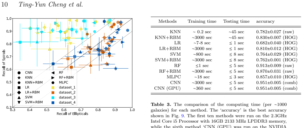
The paper's central claim is that, for binary elliptical/spiral classification from image pixels alone on Dark Energy Survey stamps, a convolutional neural network outperforms K-nearest neighbours, logistic regression, support vector machines, random forests, multi-layer perceptrons, and their restricted-Boltzmann-machine variants. With about 2,800 Galaxy Zoo 1 labelled galaxies rotated into roughly 100,000 training samples, the CNN reaches an accuracy near 0.95 with balanced data and combined raw-plus-HOG input. Raising the classification threshold to $p \geq 0.8$ lifts accuracy to about 0.987 by marking low-confidence objects as uncertain, and most of those uncertain objects look like lenticulars on DES images. The paper also claims that about 2.5 per cent of the Galaxy Zoo 1 labels in this sample are wrong, visible when DES's sharper, deeper images expose structure that SDSS lacked; after correcting those labels and retraining, the average accuracy over five runs exceeds 0.99.
Load-bearing premise
The argument assumes that the galaxies the CNN repeatedly flags as 'confirmed misclassified' truly have wrong Galaxy Zoo 1 labels, so that relabelling them and then reporting accuracy is a fair test rather than circular self-confirmation; this enters where the model's own repeated failures decide the corrected truth (Section 5.2.4).
Editorial extensions
If this is right
- A pre-trained CNN on DES-style pixel stamps can be applied directly to millions of galaxies, giving binary morphology without additional human labels.
- Balancing the training set by class is necessary when using pixel input; unbalanced sets systematically depress elliptical recall in most methods.
- The uncertainty channel, $p < 0.8$, is an inexpensive way to flag objects that need human inspection, and in practice those objects are dominated by lenticulars.
- Galaxy Zoo 1 labels carry measurable contamination, about 2.5 per cent in this sample, and machine-learning triage can flag suspects for reclassification in future surveys.
- HOG features help most pixel-based methods but not K-nearest neighbours, and their benefit largely disappears when a restricted Boltzmann machine already compresses the features.
Reading between the lines
- Because the same CNN defines which labels are 'confirmed misclassifications' and then measures its own accuracy on the corrected labels, the 0.994 figure is best read as an upper bound until independent visual confirmation of those roughly 2.5 per cent of objects.
- If the lenticular finding generalizes, the probability gap between the two softmax outputs can be used as a rough morphological axis: S0 candidates, mergers, and edge-on discs may all collect at intermediate probabilities, giving three effective classes from a binary trainer.
- A direct extension would ask whether the corrected labels also improve the non-CNN methods, since the paper retrains only the CNN after purification; the ranking of the ten methods could shift if all of them received the cleaner training set.
Signed reviews
Editorial analysis
A structured set of objections, weighed in public.
Referee Report
Summary. This paper presents a systematic comparison of ten supervised machine learning methods (including CNN, KNN, LR, SVM, RF, MLPC, and their variants with RBMs) for binary morphological classification of galaxies into ellipticals and spirals using DES imaging with Galaxy Zoo 1 (GZ1) visual labels. The authors evaluate pixel inputs, HOG features, and a CNN-specific combination input, and consistently find CNN to be the best method. The paper further investigates misclassifications, identifies lenticular galaxies as low-confidence objects, and claims that after purifying the training and test labels of ~2.5% of galaxies misclassified by GZ1, CNN reaches an average accuracy of 0.991 (best 0.994). The central claims are the CNN ranking and the >0.99 accuracy figure.
Significance. If the >0.99 accuracy claim were valid, this would be a strong benchmark for automated morphological classification on DES-like imaging and a useful guide for method selection. The paper deserves credit for a systematic, consistent comparison: a fixed 1,000-galaxy test set, three to five reruns, and ROC curves with uncertainty bands are used throughout. The rediscovery of lenticulars as uncertain objects is an interesting empirical result. However, the headline accuracy is not an unbiased measurement as presented; the method comparison and the accuracy claim must be evaluated separately, and the latter currently rests on a circular relabeling procedure and on discarding uncertain galaxies.
major comments (3)
- [Section 5.2.4, Table 8, Table 9] The reported accuracies of 0.991 and 0.994 after 'correcting' GZ1 labels are not independent measurements. The confirmed misclassifications are defined by the CNN's own repeated failures: a galaxy is 'confirmed' if it appears at least four times in total failures and at least once among high-probability failures (Table 8). These same labels are then changed in the test set and used to compute the accuracy. Because the model's disagreements define the ground truth, the evaluation is circular, and the abstract's claim of approximately 0.99 accuracy is not supported as an unbiased estimate. I recommend either independently validating the relabeled objects (e.g., by expert visual classification of the full confirmed list, not only the three unanimous-disagreement galaxies in Section 4.5) or clearly reframing the abstract and conclusions to present the corrected-label accuracy as a post-hoc consistency check rather than the model's predictive accuracy.
- [Section 5.1, Table 5, Table 9] The headline accuracy is computed only for the N_classifiable subset (p >= 0.8) and excludes 'uncertain' galaxies. For example, Table 5 reports accuracy 0.974 on 912 classifiable galaxies, while 88 of the 1,000 test galaxies are excluded; Table 9 similarly reports 0.991 on 976 galaxies with 16 uncertain. The abstract's '~0.99' is therefore conditional on discarding the hardest cases. If the uncertain galaxies are counted as errors, the full-sample accuracy is substantially lower (e.g., in Table 5, dataset 2: 912 * 0.974 / 1000 is about 0.889). The abstract and conclusions should state explicitly that the accuracy applies to the high-confidence subsample, not to the full test sample.
- [Section 5.2.4] The claimed ~2.5% misclassification rate in GZ1 is derived from the CNN-based frequency criteria, but the paper does not describe an independent verification procedure for the full 'confirmed' list (Fig. 14). The authors visually confirm three unanimous-disagreement galaxies in Section 4.5, but no such external verification is reported for the 25 or so confirmed objects. Without independent labels or a described expert inspection protocol, the misclassification rate is also a product of the CNN's behavior and is not independently established.
minor comments (5)
- [Abstract] The phrase 'or a investigation' contains a grammar error; it should be 'or an investigation'.
- [Table 5 and Table 9] The column header 'Nuncetain' appears to be a typo for 'Nuncertain'.
- [Section 2.1.1] The sentence describing the added Gaussian noise is garbled: 'it is big enough to make a detectable but change of pixel values' should be rewritten for clarity.
- [Section 5.2.4] The description of the purification procedure would benefit from a clearer account of the number of iterations: the text states 'After carrying out this purification twice,' but the preceding description of rerunning five times on each new training set is ambiguous about how the two iterations relate to the five reruns.
- [Table 3] The table footnote refers to 'the sixth method' when describing 'CNN (GPU)', but CNN (GPU) is not the sixth row; this should be corrected.
Circularity Check
Headline 0.99+ accuracy is partly circular: 'corrected' test labels are generated by the CNN's own failure criteria, and uncertain galaxies are excluded from the denominator.
-
fitted input called prediction
[Section 5.2.4, Table 8 and Table 9 (with Section 5.2.1)]
"We purify our training set by excluding the suspected misclassified galaxies then use the criteria shown in Table 8 to confirm or dismiss our suspected misclassifications... We then change the label of the confirmed misclassified galaxies in the testing set as well. ... We obtain the accuracy of 0.994 for the best model within five reruns, and the average accuracy of five reruns is 0.991."
The 'confirmed' GZ1 misclassifications are selected by the CNN's own disagreement frequency: Table 8 requires appearing at least 4 times in total failures and at least once in high-probability failures, where 'failures' mean disagreement with the GZ1 label. The new 'corrected' test labels are therefore essentially the labels the CNN tends to output. Retraining with those labels, changing the same labels in the test set, and then reporting 0.991/0.994 accuracy measures how well the CNN agrees with a ground truth partly manufactured from the CNN's own predictions. The paper presents only a few example images (Fig. 12), not an independent expert reclassification of the full confirmed list, so the corrected labels are not externally grounded.
-
other
[Section 5.1, Table 5 and Table 9 caption; compare with abstract]
"The definition of accuracy (Equation 5) and the meaning of R01 are same as in Table 4. Nclassifiable and Nuncertain are the number of testing data which are classifiable (namely p≥ 0.8) and uncertain (probabilities of both types(p) < 0.8), respectively."
The ~0.99 accuracy is computed only over the Nclassifiable subset after applying the CNN's own confidence threshold p>=0.8; the 'uncertain' galaxies (e.g. 42–88 of the 1,000 test galaxies in Table 5, and 16–19 in Table 9) are removed from the denominator. This makes the headline accuracy conditional on the classifier's own probability estimates, so the hardest cases, by the model's own judgment, do not count as errors. If those uncertain galaxies were counted as failures, the full-sample accuracy would be lower than the claimed ~0.99. The metric is therefore partly self-selected rather than a full-sample measurement.
full rationale
The comparison of the ten methods on the original GZ1 labels is a legitimate, self-contained benchmark: all methods are trained on the same augmented data and tested on the same 1,000 objects, so the conclusion that CNN outperforms the other methods is not itself circular. However, the paper's most public-facing claims—accuracy of ~0.99 and best accuracy of 0.994—come from Section 5.2.4, where test labels are changed to the CNN's own predicted classes for objects selected by the CNN's disagreement frequency, with no independent expert relabeling of the complete confirmed list. The accuracy measured after that relabeling is an internal consistency check, not an independent accuracy measurement on the original labels. The additional restriction to p>=0.8 'classifiable' galaxies removes the uncertain cases from the denominator, so the reported figure is also conditional on the model's own confidence threshold. The 0.99+ numbers should therefore be re-validated on a blind, independently labeled test sample before being accepted as evidence of near-perfect classification. No load-bearing self-citation chain or imported uniqueness theorem appears in the paper; the circularity is confined to the relabeled evaluation and the conditional accuracy reporting.
Assumptions & free parameters
free parameters (8)
- KNN k =
5
- Random Forest n_estimators =
200
- SVM nu =
not stated
- RBM hidden units and learning rate =
1024 units, lr 0.001, 500 iterations
- MLPC architecture =
2 hidden layers x 1024 units, lr 0.001
- CNN architecture =
3 conv layers (32/64/128, filters 3,3,2), pooling 2, 2 hidden x1024, dropout 0.5, lr 0.001
- Probability threshold p =
0.8
- Confirmed misclassified criteria =
appears >=4 times in total failures and >=1 in high-p failures
assumptions (4)
- domain assumption Galaxy Zoo 1 labels with over 80 percent volunteer agreement and Bamford et al. (2009) debiasing are valid ground truth for initial training and testing.
- domain assumption Rotated and Gaussian-noised copies of a galaxy image retain the same morphological class as the original.
- domain assumption DES i-band coadd images are sufficient to visually confirm the true morphology of galaxies, including cases where SDSS-based GZ1 labels are wrong.
- ad hoc to paper The frequency criteria in Table 8 identify genuine GZ1 misclassifications rather than mere CNN instabilities.
Cite this review
Pith. "Pith review of Optimising Automatic Morphological Classification of Galaxies with Machine Learning and Deep Learning using Dark Energy Survey Imaging." pith.science (2026). https://pith.science/paper/G6723AUC
@misc{pith2026190803610,
  author       = {Pith},
  title        = {Pith review of: Optimising Automatic Morphological Classification of Galaxies with Machine Learning and Deep Learning using Dark Energy Survey Imaging},
  year         = {2026},
  howpublished = {\url{https://pith.science/paper/G6723AUC}},
  note         = {Machine review of arXiv:1908.03610}
}
abstract
There are several supervised machine learning methods used for the application of automated morphological classification of galaxies; however, there has not yet been a clear comparison of these different methods using imaging data, or a investigation for maximising their effectiveness. We carry out a comparison between several common machine learning methods for galaxy classification (Convolutional Neural Network (CNN), K-nearest neighbour, Logistic Regression, Support Vector Machine, Random Forest, and Neural Networks) by using Dark Energy Survey (DES) data combined with visual classifications from the Galaxy Zoo 1 project (GZ1). Our goal is to determine the optimal machine learning methods when using imaging data for galaxy classification. We show that CNN is the most successful method of these ten methods in our study. Using a sample of $\sim$2,800 galaxies with visual classification from GZ1, we reach an accuracy of $\sim$0.99 for the morphological classification of Ellipticals and Spirals. The further investigation of the galaxies that have a different ML and visual classification but with high predicted probabilities in our CNN usually reveals an the incorrect classification provided by GZ1. We further find the galaxies having a low probability of being either spirals or ellipticals are visually Lenticulars (S0), demonstrating that supervised learning is able to rediscover that this class of galaxy is distinct from both Es and Spirals. We confirm that $\sim$2.5\% galaxies are misclassified by GZ1 in our study. After correcting these galaxies' labels, we improve our CNN performance to an average accuracy of over 0.99 (accuracy of 0.994 is our best result).
Figures


Figures from the paper (15 more)




Forward citations
Cited by 2 Pith papers
-
Deblending and Classifying Astronomical Sources with Mask R-CNN Deep Learning
A Mask R-CNN network simultaneously detects, classifies, and deblends stars and galaxies in simulated and real DECam images, achieving 92% and 98% precision at 80% recall for stars and galaxies respectively.
-
Uncertainty-Aware Deep Learning for the Ly$\alpha$ Forest: CNN-Based Absorber Detection and Characterization
A sliding-window CNN recovers Lyα absorber locations and Voigt parameters from spectra, reproducing CDDF and b–N relations on mocks and, more weakly, on UVES data.
Reference graph
Works this paper leans on
-
[1]
write newline
" write newline "" before.all 'output.state := FUNCTION fin.entry write newline FUNCTION new.block output.state before.all = 'skip after.block 'output.state := if FUNCTION new.sentence output.state after.block = 'skip output.state before.all = 'skip after.sentence 'output.state := if if FUNCTION not #0 #1 if FUNCTION and 'skip pop #0 if FUNCTION or pop #1...
-
[2]
Abbott T. M. C., et al., 2018, @doi [ ] 10.3847/1538-4365/aae9f0 , https://ui.adsabs.harvard.edu/abs/2018ApJS..239...18A 239, 18
-
[3]
Abraham R. G., van den Bergh S., Nair P., 2003, @doi [ ] 10.1086/373919 , https://ui.adsabs.harvard.edu/abs/2003ApJ...588..218A 588, 218
doi:10.1086/373919 2003
-
[4]
Avestruz C., Li N., Zhu H., Lightman M., Collett T. E., Luo W., 2019, @doi [ ] 10.3847/1538-4357/ab16d9 , https://ui.adsabs.harvard.edu/abs/2019ApJ...877...58A 877, 58
-
[6]
Ball N. M., Brunner R. J., Myers A. D., Tcheng D., 2006, @doi [ ] 10.1086/507440 , https://ui.adsabs.harvard.edu/abs/2006ApJ...650..497B 650, 497
doi:10.1086/507440 2006
-
[9]
Beck M. R., et al., 2018, @doi [ ] 10.1093/mnras/sty503 , https://ui.adsabs.harvard.edu/abs/2018MNRAS.476.5516B 476, 5516
-
[10]
M., 2006, Pattern Recognition and Machine Learning (Information Science and Statistics)
Bishop C. M., 2006, Pattern Recognition and Machine Learning (Information Science and Statistics). Springer-Verlag, Berlin, Heidelberg
work page 2006
-
[11]
P., 1997, @doi [Pattern Recognition] https://doi.org/10.1016/S0031-3203(96)00142-2 , 30, 1145
Bradley A. P., 1997, @doi [Pattern Recognition] https://doi.org/10.1016/S0031-3203(96)00142-2 , 30, 1145
Show all 71 references
-
[12]
Learn.] 10.1023/A:1010933404324 , 45, 5–32
Breiman L., 2001, @doi [Mach. Learn.] 10.1023/A:1010933404324 , 45, 5–32
2001 doi
-
[13]
Chopra P., Yadav S., 2017, @doi [Complex & Intelligent Systems] 10.1007/s40747-017-0054-8 , pp 1--11
2017 doi
-
[14]
J., 2003, @doi [ ] 10.1086/375001 , https://ui.adsabs.harvard.edu/abs/2003ApJS..147....1C 147, 1
Conselice C. J., 2003, @doi [ ] 10.1086/375001 , https://ui.adsabs.harvard.edu/abs/2003ApJS..147....1C 147, 1
2003 doi
-
[15]
pp 273--297
Cortes C., Vapnik V., 1995, in Machine Learning. pp 273--297
1995
-
[16]
Cover T., Hart P., 1967, @doi [IEEE Transactions on Information Theory] 10.1109/TIT.1967.1053964 , 13, 21
1967
-
[17]
J., 2007, k-Nearest Neighbour Classifiers
Cunningham P., Delany S. J., 2007, k-Nearest Neighbour Classifiers
2007
-
[18]
pp 886--893 vol
Dalal N., Triggs B., 2005, in 2005 IEEE Computer Society Conference on Computer Vision and Pattern Recognition (CVPR'05). pp 886--893 vol. 1, @doi 10.1109/CVPR.2005.177
2005 doi
-
[19]
W., Dambre J., 2015, @doi [ ] 10.1093/mnras/stv632 , https://ui.adsabs.harvard.edu/abs/2015MNRAS.450.1441D 450, 1441
Dieleman S., Willett K. W., Dambre J., 2015, @doi [ ] 10.1093/mnras/stv632 , https://ui.adsabs.harvard.edu/abs/2015MNRAS.450.1441D 450, 1441
2015 doi
-
[20]
L., 2018, @doi [ ] 10.1093/mnras/sty338 , https://ui.adsabs.harvard.edu/abs/2018MNRAS.476.3661D 476, 3661
Dom \' nguez S \'a nchez H., Huertas-Company M., Bernardi M., Tuccillo D., Fischer J. L., 2018, @doi [ ] 10.1093/mnras/sty338 , https://ui.adsabs.harvard.edu/abs/2018MNRAS.476.3661D 476, 3661
2018 doi
-
[21]
Drlica-Wagner A., et al., 2018, @doi [ ] 10.3847/1538-4365/aab4f5 , https://ui.adsabs.harvard.edu/abs/2018ApJS..235...33D 235, 33
2018 doi
-
[22]
Dubath P., et al., 2011, @doi [ ] 10.1111/j.1365-2966.2011.18575.x , https://ui.adsabs.harvard.edu/abs/2011MNRAS.414.2602D 414, 2602
2011
-
[23]
M., Elyan E., 2014, @doi [Systems Science & Control Engineering] 10.1080/21642583.2014.956265 , 2, 602
Fawagreh K., Gaber M. M., Elyan E., 2014, @doi [Systems Science & Control Engineering] 10.1080/21642583.2014.956265 , 2, 602
2014
-
[24]
Fawcett T., 2006, @doi [Pattern Recognition Letters] https://doi.org/10.1016/j.patrec.2005.10.010 , 27, 861
2006 doi
-
[25]
L., 1989, International Statistical Review / Revue Internationale de Statistique, 57, 238
Fix E., Hodges J. L., 1989, International Statistical Review / Revue Internationale de Statistique, 57, 238
1989
-
[26]
Flaugher B., et al., 2015, @doi [ ] 10.1088/0004-6256/150/5/150 , https://ui.adsabs.harvard.edu/abs/2015AJ....150..150F 150, 150
2015 doi
-
[27]
Fukushima K., 1975, Biological Cybernetics, 20, 121
1975
-
[28]
Fukushima K., 1980, @doi [Biological Cybernetics] 10.1007/bf00344251 , 36, 193
1980 doi
-
[29]
Fukushima K., Miyake S., Ito T., 1983, @doi [IEEE Transactions on Systems, Man, and Cybernetics] 10.1109/TSMC.1983.6313076 , SMC-13, 826
1983
-
[31]
N., Lolling S
Goderya S. N., Lolling S. M., 2002, @doi [ ] 10.1023/A:1015193432240 , https://ui.adsabs.harvard.edu/abs/2002Ap&SS.279..377G 279, 377
2002 doi
-
[32]
E., 2002, @doi [Neural Comput.] 10.1162/089976602760128018 , 14, 1771–1800
Hinton G. E., 2002, @doi [Neural Comput.] 10.1162/089976602760128018 , 14, 1771–1800
2002 doi
-
[33]
E., Sun Y., Davey N., 2018, @doi [ ] 10.1093/mnras/stx2351 , https://ui.adsabs.harvard.edu/abs/2018MNRAS.473.1108H 473, 1108
Hocking A., Geach J. E., Sun Y., Davey N., 2018, @doi [ ] 10.1093/mnras/stx2351 , https://ui.adsabs.harvard.edu/abs/2018MNRAS.473.1108H 473, 1108
2018 doi
-
[34]
Department of Computer Science, National Taiwan University, http://www.csie.ntu.edu.tw/ cjlin/papers.html
Hsu C.-W., Chang C.-C., Lin C.-J., 2003, Technical report, A Practical Guide to Support Vector Classification, http://www.csie.ntu.edu.tw/ cjlin/papers.html . Department of Computer Science, National Taiwan University, http://www.csie.ntu.edu.tw/ cjlin/papers.html
2003
-
[35]
P., 1926, @doi [ ] 10.1086/143018 , https://ui.adsabs.harvard.edu/abs/1926ApJ....64..321H 64, 321
Hubble E. P., 1926, @doi [ ] 10.1086/143018 , https://ui.adsabs.harvard.edu/abs/1926ApJ....64..321H 64, 321
1926 doi
-
[36]
Huertas-Company M., Rouan D., Tasca L., Soucail G., Le F \`e vre O., 2008, @doi [ ] 10.1051/0004-6361:20078625 , https://ui.adsabs.harvard.edu/abs/2008A&A...478..971H 478, 971
2008 doi
-
[37]
Huertas-Company M., et al., 2009, @doi [ ] 10.1051/0004-6361/200811255 , https://ui.adsabs.harvard.edu/abs/2009A&A...497..743H 497, 743
2009 doi
-
[38]
Huertas-Company M., Aguerri J. A. L., Bernardi M., Mei S., S \'a nchez Almeida J., 2011, @doi [ ] 10.1051/0004-6361/201015735 , https://ui.adsabs.harvard.edu/abs/2011A&A...525A.157H 525, A157
2011 doi
-
[39]
Huertas-Company M., et al., 2015, @doi [ ] 10.1088/0067-0049/221/1/8 , https://ui.adsabs.harvard.edu/abs/2015ApJS..221....8H 221, 8
2015 doi
-
[40]
Huertas-Company M., et al., 2018, @doi [ ] 10.3847/1538-4357/aabfed , https://ui.adsabs.harvard.edu/abs/2018ApJ...858..114H 858, 114
2018 doi
-
[41]
M., Hogg D
Huppenkothen D., Heil L. M., Hogg D. W., Mueller A., 2017, @doi [ ] 10.1093/mnras/stw3190 , https://ui.adsabs.harvard.edu/abs/2017MNRAS.466.2364H 466, 2364
2017 doi
-
[42]
M., Hegadi R
Kamble P. M., Hegadi R. S., 2015, @doi [Procedia Computer Science] https://doi.org/10.1016/j.procs.2015.03.137 , 45, 266
2015 doi
-
[43]
Kov \'a cs A., Szapudi I., 2015, @doi [ ] 10.1093/mnras/stv063 , https://ui.adsabs.harvard.edu/abs/2015MNRAS.448.1305K 448, 1305
2015 doi
-
[44]
D., Polsterer K., Hoecker M., 2015, @doi [ ] 10.1051/0004-6361/201424801 , https://ui.adsabs.harvard.edu/abs/2015A&A...576A.132K 576, A132
K \"u gler S. D., Polsterer K., Hoecker M., 2015, @doi [ ] 10.1051/0004-6361/201424801 , https://ui.adsabs.harvard.edu/abs/2015A&A...576A.132K 576, A132
2015 doi
-
[45]
J., Storrie-Lombardi M
Lahav O., Naim A., Sodr \'e L. J., Storrie-Lombardi M. C., 1996, @doi [ ] 10.1093/mnras/283.1.207 , https://ui.adsabs.harvard.edu/abs/1996MNRAS.283..207L 283, 207
1996 doi
-
[46]
Lecun Y., Bottou L., Bengio Y., Haffner P., 1998, @doi [Proceedings of the IEEE] 10.1109/5.726791 , 86, 2278
1998 doi
-
[47]
J., et al., 2008, @doi [ ] 10.1111/j.1365-2966.2008.13689.x , https://ui.adsabs.harvard.edu/abs/2008MNRAS.389.1179L 389, 1179
Lintott C. J., et al., 2008, @doi [ ] 10.1111/j.1365-2966.2008.13689.x , https://ui.adsabs.harvard.edu/abs/2008MNRAS.389.1179L 389, 1179
2008
-
[48]
Lintott C., et al., 2011, @doi [ ] 10.1111/j.1365-2966.2010.17432.x , https://ui.adsabs.harvard.edu/abs/2011MNRAS.410..166L 410, 166
2011
-
[49]
H., Hakala P
Maehoenen P. H., Hakala P. J., 1995, @doi [ ] 10.1086/309697 , https://ui.adsabs.harvard.edu/abs/1995ApJ...452L..77M 452, L77
1995 doi
-
[50]
Chapman and Hall/CRC Monographs on Statistics and Applied Probability Series, Chapman & Hall, http://books.google.com/books?id=h9kFH2\_FfBkC
McCullagh P., Nelder J., 1989, Generalized Linear Models, Second Edition. Chapman and Hall/CRC Monographs on Statistics and Applied Probability Series, Chapman & Hall, http://books.google.com/books?id=h9kFH2\_FfBkC
1989
-
[51]
B., et al., 2019, @doi [ ] 10.1051/0004-6361/201832797 , https://ui.adsabs.harvard.edu/abs/2019A&A...625A.119M 625, A119
Metcalf R. B., et al., 2019, @doi [ ] 10.1051/0004-6361/201832797 , https://ui.adsabs.harvard.edu/abs/2019A&A...625A.119M 625, A119
2019 doi
-
[52]
J., Storrie-Lombardi M
Naim A., Lahav O., Sodre L. J., Storrie-Lombardi M. C., 1995, @doi [ ] 10.1093/mnras/275.3.567 , https://ui.adsabs.harvard.edu/abs/1995MNRAS.275..567N 275, 567
1995 doi
-
[53]
C., Stockwell E
Odewahn S. C., Stockwell E. B., Pennington R. L., Humphreys R. M., Zumach W. A., 1992, @doi [ ] 10.1086/116063 , https://ui.adsabs.harvard.edu/abs/1992AJ....103..318O 103, 318
1992 doi
-
[54]
Orr M. J. L., Science C. F. C., 1996, Technical report, Introduction to radial basis function networks
1996
-
[55]
arXiv:1201.0490
Pedregosa F., et al., 2012, arXiv e-prints, https://ui.adsabs.harvard.edu/abs/2012arXiv1201.0490P p. arXiv:1201.0490
2012 arXiv
-
[56]
L., Gieseke F., Kramer O., 2012, Galaxy Classification without Feature Extraction
Polsterer K. L., Gieseke F., Kramer O., 2012, Galaxy Classification without Feature Extraction . p. 561
2012
-
[57]
Powers D. M. W., 2011, Journal of Machine Learning Technologies, 2, 37
2011
-
[58]
Rosenblatt F., 1958, Psychological Review, pp 65--386
1958
-
[59]
E., Hinton G
Rumelhart D. E., Hinton G. E., Williams R. J., 1986, @doi [ ] 10.1038/323533a0 , https://ui.adsabs.harvard.edu/abs/1986Natur.323..533R 323, 533
1986 doi
-
[60]
ICML ’07
Salakhutdinov R., Mnih A., Hinton G., 2007, in Proceedings of the 24th International Conference on Machine Learning. ICML ’07. Association for Computing Machinery, New York, NY, USA, p. 791–798, @doi 10.1145/1273496.1273596 , https://doi.org/10.1145/1273496.1273596
2007
-
[61]
J., 2001, Learning with Kernels: Support Vector Machines, Regularization, Optimization, and Beyond
Scholkopf B., Smola A. J., 2001, Learning with Kernels: Support Vector Machines, Regularization, Optimization, and Beyond. MIT Press, Cambridge, MA, USA
2001
-
[62]
Shamir L., 2009, @doi [ ] 10.1111/j.1365-2966.2009.15366.x , https://ui.adsabs.harvard.edu/abs/2009MNRAS.399.1367S 399, 1367
2009
-
[63]
D., Fukunaga K., 1981, IEEE Trans
Short R. D., Fukunaga K., 1981, IEEE Trans. Information Theory, 27, 622
1981
-
[64]
Shu C., Ding X., Fang C., 2011, @doi [Tsinghua Science and Technology] 10.1016/S1007-0214(11)70032-3 , 16, 216
2011 doi
-
[65]
MIT Press, Cambridge, MA, USA, p
Smolensky P., 1986, Information Processing in Dynamical Systems: Foundations of Harmony Theory. MIT Press, Cambridge, MA, USA, p. 194–281
1986
-
[66]
Sreejith S., et al., 2018, @doi [ ] 10.1093/mnras/stx2976 , https://ui.adsabs.harvard.edu/abs/2018MNRAS.474.5232S 474, 5232
2018 doi
-
[67]
C., Lahav O., Sodre L
Storrie-Lombardi M. C., Lahav O., Sodre L. J., Storrie-Lombardi L. J., 1992, @doi [ ] 10.1093/mnras/259.1.8P , https://ui.adsabs.harvard.edu/abs/1992MNRAS.259P...8S 259, 8P
1992 doi
-
[68]
M., 1950, @doi [Mind] 10.1093/mind/LIX.236.433 , LIX, 433
TURING A. M., 1950, @doi [Mind] 10.1093/mind/LIX.236.433 , LIX, 433
1950 doi
-
[69]
N., 1995, The Nature of Statistical Learning Theory
Vapnik V. N., 1995, The Nature of Statistical Learning Theory. Springer-Verlag, Berlin, Heidelberg
1995
-
[70]
M., Djorgovski S., 1995, @doi [ ] 10.1086/117459 , https://ui.adsabs.harvard.edu/abs/1995AJ....109.2401W 109, 2401
Weir N., Fayyad U. M., Djorgovski S., 1995, @doi [ ] 10.1086/117459 , https://ui.adsabs.harvard.edu/abs/1995AJ....109.2401W 109, 2401
1995 doi
-
[71]
Werbos P., John P., 1974
1974
-
[72]
W., et al., 2013, @doi [ ] 10.1093/mnras/stt1458 , https://ui.adsabs.harvard.edu/abs/2013MNRAS.435.2835W 435, 2835
Willett K. W., et al., 2013, @doi [ ] 10.1093/mnras/stt1458 , https://ui.adsabs.harvard.edu/abs/2013MNRAS.435.2835W 435, 2835
2013 doi
-
[73]
Y., 2003, in In ICML 2003 Workshop on Learning from Imbalanced Data Sets
Wu G., Chang E. Y., 2003, in In ICML 2003 Workshop on Learning from Imbalanced Data Sets. pp 49--56
2003
-
[74]
Zanaty E., 2012, @doi [Egyptian Informatics Journal] https://doi.org/10.1016/j.eij.2012.08.002 , 13, 177
2012 doi
-
[75]
de la Calleja J., Fuentes O., 2004, @doi [ ] 10.1111/j.1365-2966.2004.07442.x , https://ui.adsabs.harvard.edu/abs/2004MNRAS.349...87D 349, 87
2004
Reviewed August 14, 2026 · model on record in the stance chip above.
Discussion (0). Continue with ORCID to comment.