Target-Oriented Statistical Compression: Sufficiency, Reverse Martingales, and Sequential Monitoring
Pith reviewed 2026-06-29 16:00 UTC · model grok-4.3
The pith
The conditional target process is a reverse martingale under decreasing filtrations from compression maps, unifying exact sufficiency with approximate statistical summaries.
A machine-rendered reading of the paper's core claim, the machinery that carries it, and where it could break.
Core claim
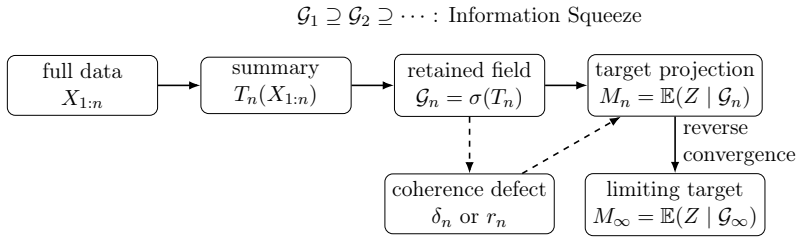
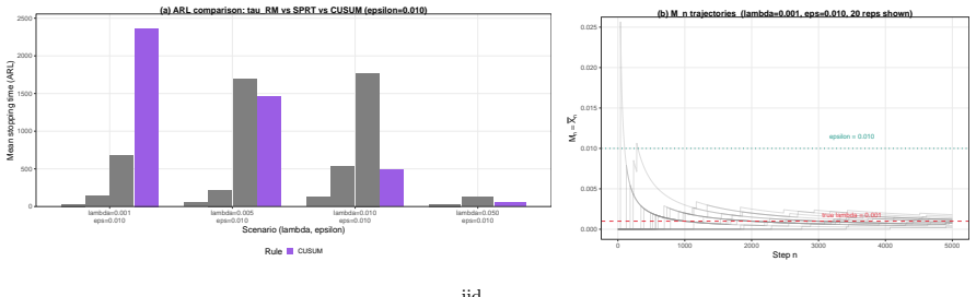
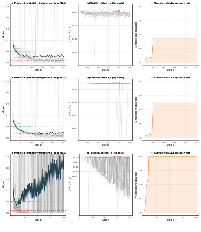
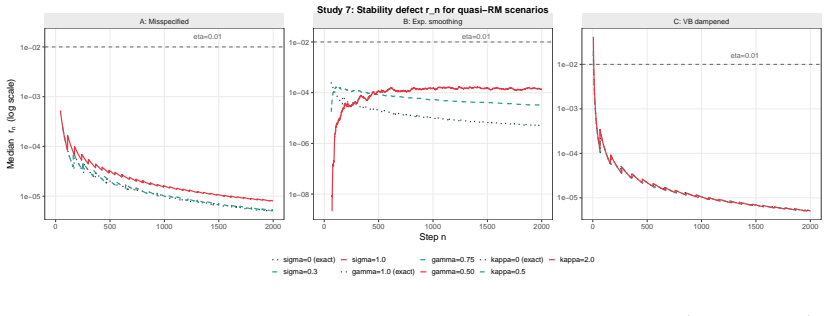
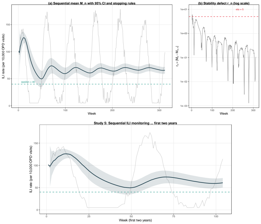
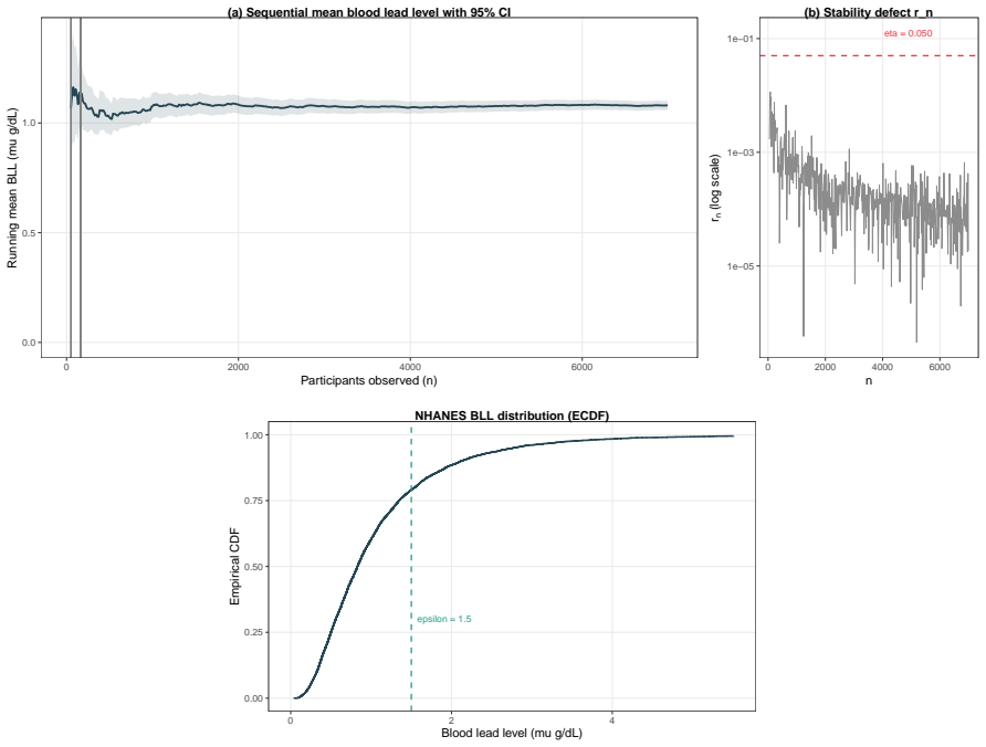
When (G_n) is a decreasing filtration generated by compression maps T_n, the process M_n = E(Z | G_n) is a reverse martingale with limit M_infty = E(Z | G_infty). Exact sufficiency is lossless compression in this sense, while approximate summaries yield reverse quasi-martingale defects that quantify the loss of coherence across compression levels. The quantity r_n = |M_n - M_{n-1}| acts as an observable proxy for stability in applications such as boundary degeneracy in sequential binary problems.
What carries the argument
The conditional target process M_n = E(Z | G_n), where G_n = sigma(T_n) is the sigma-field retained by the compression map T_n; it supplies the reverse-martingale property that turns exact sufficiency into lossless preservation of the target and turns approximation error into a measurable defect.
If this is right
- Exact sufficiency corresponds to the case where the quasi-martingale defect is identically zero.
- Approximate summaries such as penalized estimators or neural hidden states produce strictly positive defects that measure coherence loss across successive compression levels.
- The observable diagnostic r_n = |M_n - M_{n-1}| supplies a practical stability proxy for assessing boundary claims in sequential monitoring.
- The same reverse-martingale structure extends directly to Gaussian, Poisson, and general quasi-martingale monitoring problems.
Where Pith is reading between the lines
- The framework implies that one could design monitoring rules by directly bounding the observed defects r_n rather than relying solely on theoretical probability bounds.
- The requirement of a decreasing filtration suggests that the order in which successive summaries are applied matters and may need explicit verification in practice.
- The unification points to analogous constructions in online learning where successive representations compress history for a downstream prediction target.
Load-bearing premise
The sigma-fields generated by successive compression maps must form a decreasing filtration.
What would settle it
A concrete sequence of compression maps that produces a strictly decreasing filtration yet yields conditional expectations M_n that fail to satisfy the reverse-martingale equality E(M_n | G_{n+1}) = M_{n+1}.
Figures
read the original abstract
Statistical procedures rarely retain all features of the observed data. A sufficient statistic removes information irrelevant to a parameter; a maximum likelihood estimate compresses an empirical objective into an optimizing point; and a hidden state in a sequential model compresses past observations into a learned representation. This article develops these practices under the unified notion of \emph{target-oriented statistical compression}: a useful summary preserves what matters for an inferential, predictive, or decision-relevant target, rather than every detail of the realized data path. The central object is the conditional target process \(M_n=\E(Z\given\G_n)\), where \(Z\) is the target and \(\G_n=\sigma(T_n)\) is the information retained by the compression map \(T_n\). When \((\G_n)\) is a decreasing filtration, \((M_n)\) is a reverse martingale with limit \(M_\infty=\E(Z\given\G_\infty)\). Exact sufficiency corresponds to lossless compression, while approximate summaries such as penalized estimators, principal components, and neural-network hidden states produce reverse quasi-martingale defects measuring coherence loss across compression levels. The diagnostic \(r_n=|M_n-M_{n-1}|\) is treated as an observable stability proxy, not as an unbiased estimator of the theoretical defect. Boundary degeneracy in sequential binary problems is developed as a central application. Practical boundary claims require joint assessment of boundary closeness, uncertainty control, and trajectory stability. The companion paper \citet{chang2025rm} develops the corresponding stopping procedures, finite-sample bounds, and numerical evidence; the present paper provides the broader theoretical infrastructure and extends the framework to Gaussian, Poisson, and quasi-martingale monitoring problems.
Editorial analysis
A structured set of objections, weighed in public.
Referee Report
Summary. The paper develops target-oriented statistical compression via the conditional target process M_n = E(Z | G_n), where G_n = sigma(T_n) for a compression map T_n. It claims that when (G_n) is a decreasing filtration, (M_n) is a reverse martingale with limit M_infty = E(Z | G_infty). Exact sufficiency is lossless compression; approximate summaries (penalized estimators, principal components, neural hidden states) produce reverse quasi-martingale defects that measure coherence loss. The observable diagnostic r_n = |M_n - M_{n-1}| is a stability proxy. The framework is applied to boundary degeneracy in sequential binary problems and extended to Gaussian, Poisson, and quasi-martingale monitoring, with a companion paper supplying stopping procedures and numerics.
Significance. If the reverse-martingale property and defect interpretation hold under the paper's compression maps, the work supplies a unified martingale-based account of information retention for inference and prediction. This could furnish new diagnostics for coherence across compression levels in sequential and high-dimensional settings, with the boundary-monitoring application offering a concrete test case. The explicit separation of the theoretical infrastructure from the companion paper's finite-sample results is a structural strength.
major comments (1)
- [Abstract] Abstract (central claim paragraph): The reverse-martingale property is asserted to hold precisely when (G_n) is decreasing, yet the manuscript supplies no argument that G_n = sigma(T_n) satisfies G_{n+1} ⊆ G_n for the listed compression maps (penalized estimators, PCs, neural hidden states). If the maps are constructed independently at each level, the nesting fails and the quasi-martingale defect loses its interpretation as a coherence-loss measure. This is load-bearing for the unification claim.
Simulated Author's Rebuttal
We thank the referee for the careful reading and for identifying this load-bearing point on the filtration nesting. We respond below and will revise accordingly.
read point-by-point responses
-
Referee: [Abstract] Abstract (central claim paragraph): The reverse-martingale property is asserted to hold precisely when (G_n) is decreasing, yet the manuscript supplies no argument that G_n = sigma(T_n) satisfies G_{n+1} ⊆ G_n for the listed compression maps (penalized estimators, PCs, neural hidden states). If the maps are constructed independently at each level, the nesting fails and the quasi-martingale defect loses its interpretation as a coherence-loss measure. This is load-bearing for the unification claim.
Authors: We agree that the manuscript states the reverse-martingale property conditionally on (G_n) being decreasing but supplies no explicit argument that the listed compression maps induce G_{n+1} ⊆ G_n. The referee is correct that independent per-level construction would break the nesting and thereby weaken the defect interpretation. In the sequential-monitoring applications that form the paper's central test case, the maps are constructed recursively (e.g., successive neural hidden states or cumulative penalized estimates), which by design yields the required nesting. For the more general classes (penalized estimators, PCs), we will add a short clarifying subsection that (i) states the nesting assumption explicitly and (ii) supplies concrete recursive constructions under which it holds. This revision will be made in both the abstract and the main text so that the coherence-loss reading of the quasi-martingale defects is fully supported. revision: yes
Circularity Check
No significant circularity; derivation applies standard reverse-martingale property under explicit assumption
full rationale
The paper states the reverse-martingale property of M_n = E(Z | G_n) precisely when (G_n) is decreasing, which is a textbook fact from probability theory rather than a derived claim. It then defines G_n = σ(T_n) for compression maps and treats the decreasing-filtration condition as an assumption required for the property to hold. No equation reduces a 'prediction' or central result to a fitted parameter by construction, no self-citation is invoked to justify uniqueness or an ansatz, and the quasi-martingale defect is introduced definitionally from the conditional expectation process. The framework is therefore self-contained against external benchmarks; the companion paper citation covers applications only.
Axiom & Free-Parameter Ledger
axioms (2)
- standard math Z is integrable so that the conditional expectation E(Z | G_n) exists for each n.
- domain assumption The sequence of sigma-fields (G_n) is decreasing.
Reference graph
Works this paper leans on
-
[1]
Albert, A. and Anderson, J.\,A. (1984). On the existence of maximum likelihood estimates in logistic regression models. Biometrika, 71(1), 1--10. doi:10.1093/biomet/71.1.1 https://doi.org/10.1093/biomet/71.1.1
-
[2]
Björk, T. and Johansson, B. (1996). Parameter estimation and reverse martingales. Stochastic Processes and their Applications, 63(2), 235--263. doi:10.1016/0304-4149(96)00080-4 https://doi.org/10.1016/0304-4149(96)00080-4
-
[3]
Chakraborty, B. and Moodie, E.\,E.\,M. (2013). Statistical Methods for Dynamic Treatment Regimes. Springer, New York. doi:10.1007/978-1-4614-7428-9 https://doi.org/10.1007/978-1-4614-7428-9
-
[4]
Chang, Y.-c.\,I. (2026). Practical boundary degeneracy and reverse-martingale limits in sequential binary models. Preprint, arXiv:2605.02274 [stat.ME] https://arxiv.org/abs/2605.02274
work page internal anchor Pith review Pith/arXiv arXiv 2026
-
[5]
Clopper, C.\,J. and Pearson, E.\,S. (1934). The use of confidence or fiducial limits illustrated in the case of the binomial. Biometrika, 26(4), 404--413. doi:10.1093/biomet/26.4.404 https://doi.org/10.1093/biomet/26.4.404
-
[6]
Doob, J.\,L. (1953). Stochastic Processes. John Wiley & Sons, New York
1953
-
[7]
Durrett, R. (2019). Probability: Theory and Examples (5th ed.). Cambridge University Press, Cambridge. doi:10.1017/9781108591034 https://doi.org/10.1017/9781108591034
-
[8]
Firth, D. (1993). Bias reduction of maximum likelihood estimates. Biometrika, 80(1), 27--38. doi:10.1093/biomet/80.1.27 https://doi.org/10.1093/biomet/80.1.27
-
[9]
Fisher, R.\,A. (1922). On the mathematical foundations of theoretical statistics. Philosophical Transactions of the Royal Society A, 222, 309--368
1922
-
[10]
Fong, E., Holmes, C., and Walker, S.\,G. (2023). Martingale posterior distributions. Journal of the Royal Statistical Society: Series B, 85(5), 1357--1391. doi:10.1093/jrsssb/qkad005 https://doi.org/10.1093/jrsssb/qkad005
-
[11]
Gelman, A., Jakulin, A., Pittau, M.\,G., and Su, Y.-S. (2008). A weakly informative default prior distribution for logistic and other regression models. The Annals of Applied Statistics, 2(4), 1360--1383. doi:10.1214/08-AOAS191 https://doi.org/10.1214/08-AOAS191
-
[12]
Goodfellow, I., Bengio, Y., and Courville, A. (2016). Deep Learning. MIT Press, Cambridge, MA
2016
-
[13]
Heinze, G. and Schemper, M. (2002). A solution to the problem of separation in logistic regression. Statistics in Medicine, 21(16), 2409--2419. doi:10.1002/sim.1047 https://doi.org/10.1002/sim.1047
-
[14]
and Schmidhuber, J
Hochreiter, S. and Schmidhuber, J. (1997). Long short-term memory. Neural Computation, 9(8), 1735--1780
1997
-
[15]
Howard, S.\,R., Ramdas, A., McAuliffe, J., and Sekhon, J. (2021). Time-uniform, nonparametric, nonasymptotic confidence sequences. The Annals of Statistics, 49(2), 1055--1080. doi:10.1214/20-AOS1991 https://doi.org/10.1214/20-AOS1991
-
[16]
Kallenberg, O. (2002). Foundations of Modern Probability (2nd ed.). Springer, New York
2002
-
[17]
and Casella, G
Lehmann, E.\,L. and Casella, G. (1998). Theory of Point Estimation (2nd ed.). Springer, New York
1998
-
[18]
Murphy, S.\,A. (2003). Optimal dynamic treatment regimes. Journal of the Royal Statistical Society: Series B, 65(2), 331--355. doi:10.1111/1467-9868.00389 https://doi.org/10.1111/1467-9868.00389
-
[19]
NHANES 2017--2018: Laboratory Procedures Manual
National Center for Health Statistics (2020). NHANES 2017--2018: Laboratory Procedures Manual. National Center for Health Statistics, Centers for Disease Control and Prevention, U.S. Department of Health and Human Services, Hyattsville, MD. https://wwwn.cdc.gov/Nchs/Nhanes/2017-2018/PBCD_J.htm
2020
-
[20]
Robins, J.\,M. (2004). Optimal structural nested models for optimal sequential decisions. In D.\,Y. Lin and P.\,J. Heagerty (eds.), Proceedings of the Second Seattle Symposium in Biostatistics, Lecture Notes in Statistics, vol. 179, pp. 189--326. Springer, New York. doi:10.1007/978-1-4419-9076-1\_11 https://doi.org/10.1007/978-1-4419-9076-1_11
-
[21]
Robbins, H. (1970). Statistical methods related to the law of the iterated logarithm. The Annals of Mathematical Statistics, 41(5), 1397--1409. doi:10.1214/aoms/1177696786 https://doi.org/10.1214/aoms/1177696786
-
[22]
Siegmund, D. (1985). Sequential Analysis: Tests and Confidence Intervals. Springer, New York. doi:10.1007/978-1-4613-9549-7 https://doi.org/10.1007/978-1-4613-9549-7
-
[23]
Ville, J. (1939). \'E tude Critique de la Notion de Collectif . Gauthier-Villars, Paris
1939
-
[24]
Wald, A. (1945). Sequential tests of statistical hypotheses. The Annals of Mathematical Statistics, 16(2), 117--186. doi:10.1214/aoms/1177731118 https://doi.org/10.1214/aoms/1177731118
-
[25]
Wald, A. (1947). Sequential Analysis. John Wiley & Sons, New York
1947
-
[26]
Wald, A. and Wolfowitz, J. (1948). Optimum character of the sequential probability ratio test. The Annals of Mathematical Statistics, 19(3), 326--339. doi:10.1214/aoms/1177730197 https://doi.org/10.1214/aoms/1177730197
-
[27]
Waudby-Smith, I. and Ramdas, A. (2023). Estimating means of bounded random variables by betting. Journal of the Royal Statistical Society: Series B, 85(1), 1--26. doi:10.1093/jrsssb/qkac007 https://doi.org/10.1093/jrsssb/qkac007
-
[28]
Williams, D. (1991). Probability with Martingales. Cambridge University Press, Cambridge
1991
discussion (0)
Sign in with ORCID, Apple, or X to comment. Anyone can read and Pith papers without signing in.