REVIEW 1 major objections 4 minor 67 references
Finite-difference time-domain simulation of strong-field ionization: Perfectly matched layer approach
T0 review · 1 major / 4 minor · reviewed 2026-08-14 · deepseek-v4-flash
Pith's one-line read A perfectly matched layer in the velocity gauge reproduces the exact interior wave function for short-range strong-field ionization, cutting the simulation domain from 8000 to 120 atomic units.
desk verdict Solid PML-for-Schrodinger paper with a believable core result and an overstated ECS comparison; worth refereeing after the ECS comparison is fixed. read the letter →
The pith
A machine-rendered reading of the paper's core claim, the machinery that carries it, and where it could break.
The reading
What carries the argument
The central object is the PML coordinate transformation $x \to x + i\sigma_0 \int_{R_0}^{x} f(x') dx'$ outside the interior, acting only on spatial derivatives: $\partial_x \to c(x)\partial_x$ with $c(x)=1/[1+i\sigma_0 f(x)]$. Inside $|x|\le R_0$, $c=1$ and the original Schrödinger equation is recovered; outside, the complex stretch turns outgoing waves into decaying exponentials while ideally causing no reflection at the interface, so a Dirichlet boundary deep in the layer is harmless. The choice of absorption function $f$ (square, cubic, near-singular, or tanh-based) controls how gently the absorption turns on, and the paper shows that slowly growing $f$ yields smaller reflection errors at the cost of slower convergence.
What would settle it
Propagate the velocity-gauge FDTD-PML for the same $\delta$-potential at a field amplitude outside the tested range (e.g., $E_0=0.5$ a.u. at $\omega=0.52$ a.u., or a few-cycle pulse with a nonzero carrier-envelope phase), compare the interior wave function to a reference solution on a domain of several thousand atomic units, and check whether the interior error at $t=200$ a.u. remains near $10^{-15}$; a jump of several orders of magnitude would show that the PML's absorption of the time-dependent interaction is parameter-dependent.
Extended reading notes
Core claim
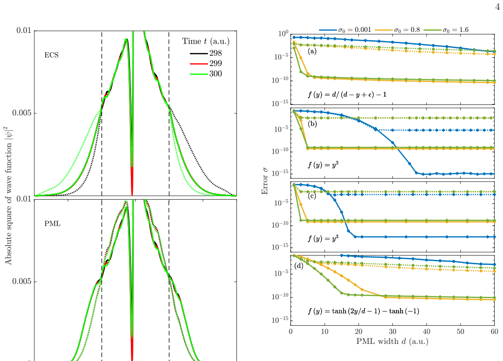
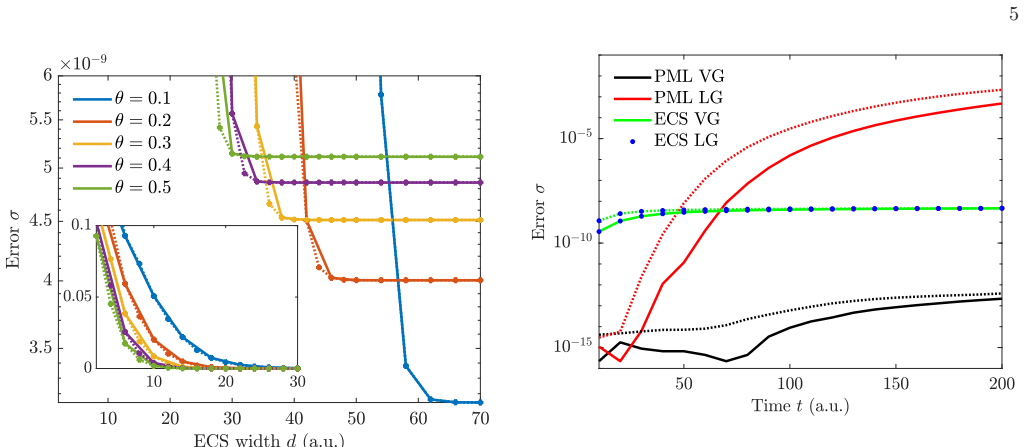
The central claim is that a perfectly matched layer implemented in the velocity gauge within a second-order finite-difference time-domain scheme reproduces the exact wave function in the interior region for an electron bound to a short-range potential driven by a strong monochromatic field. Using the square absorption function $f(y)=y^2$ with absorption strength $\sigma_0=0.001$, the error inside $|x|\le 20$ a.u. reaches $\sim 10^{-15}$ at $t=200$ a.u. with an absorbing layer of width $d=40$ a.u., i.e., a total domain of 120 a.u. instead of the 8000 a.u. needed with Dirichlet boundaries. The same comparison shows the velocity-gauge PML beats exterior complex scaling implemented with the same finite-difference formulas by several orders of magnitude. The paper further claims that the length-gauge PML introduces much larger interior errors, that slowly growing absorption functions are preferable, and that at very low frequencies the length-gauge PML is the only one of the four methods that remains numerically stable.
Load-bearing premise
The PML is derived from a modal analysis for a potential that is constant in space and time, but the paper applies the same coordinate stretch to the explicitly time-dependent velocity-gauge interaction $\mathbf p\cdot\mathbf A(t)$, and the perfect-absorption property for that term is not formally justified—only numerical agreement with a large-domain reference is offered as evidence.
Editorial extensions
If this is right
- Strong-field ionization of short-range potentials can be simulated accurately on domains two orders of magnitude smaller than with plain Dirichlet boundaries, reducing memory and computation time.
- For short-range potentials, velocity-gauge PML is the preferred absorber over ECS within finite-difference schemes, since ECS errors are several orders of magnitude larger.
- Length-gauge PML must be avoided at moderate and high frequencies, where it introduces large interior errors, but it becomes the only stable option at very low frequencies.
- Absorption functions that grow slowly reduce reflection errors at the cost of needing wider layers, and a square absorption function already reaches $10^{-15}$ with $d\approx 40$ a.u.
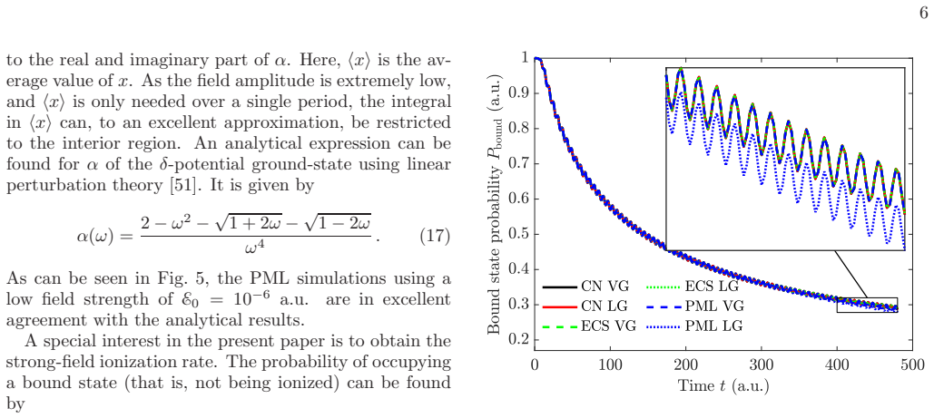
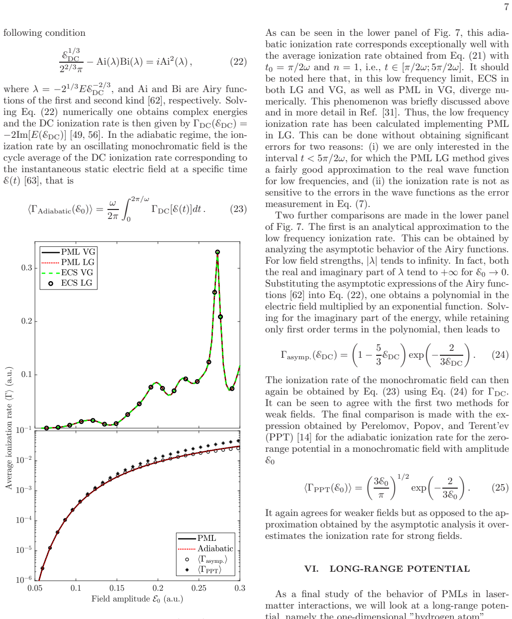
- The scheme reproduces known analytic results for the polarizability and for adiabatic ionization rates of the $\delta$-potential, indicating that physical observables remain reliable even though the wave function is absorbed.
Reading between the lines
- The formal gap between the time-independent derivation and the time-dependent $\mathbf p\cdot\mathbf A(t)$ term suggests the velocity-gauge PML advantage may not survive for arbitrary pulse shapes; scanning field amplitudes, frequencies, and carrier-envelope phases against a large-domain reference would map where the $10^{-15}$ accuracy holds.
- Because slowly growing absorption functions reduce reflection, a non-uniform grid in the absorption layer, analogous to what the paper notes for ECS, could make very wide PML layers cheap and might improve accuracy for long-range potentials where PML is currently inferior.
- The low-frequency stability of only the length-gauge PML suggests a practical hybrid: use velocity-gauge PML at moderate and high frequencies and switch to length-gauge PML in the adiabatic regime, combining the best accuracy with stability.
- Extending the scheme to two and three dimensions would open a direct path to the exciton-dissociation problems the paper motivates; the long-range potential results caution that the PML would need a tail-aware treatment or a hybrid with ECS.
Signed reviews
Editorial analysis
A structured set of objections, weighed in public.
Referee Report
Summary. The manuscript develops a finite-difference time-domain (FDTD) Crank-Nicolson solver for the one-dimensional time-dependent Schrödinger equation with perfectly matched layers (PMLs), targeting strong-field ionization of an electron bound by a short-range potential. The PML is implemented by transforming spatial derivatives while leaving the potential untransformed, and the scheme is tested in both velocity and length gauges. The paper compares absorption functions, measures the interior error against a converged large-domain reference, compares PML with exterior complex scaling (ECS) in both gauges, and validates observables against analytical results: the frequency-dependent polarizability, the adiabatic Airy-function ionization rate, an asymptotic low-field expression, and the PPT formula. The central claims are that velocity-gauge PML reproduces the exact wave function in the interior to near machine precision with a domain of about 120 a.u. instead of 8000 a.u. without absorbers, that PML outperforms ECS for short-range potentials when both are implemented in finite differences, and that ECS remains preferable for long-range potentials.
Significance. The core numerical demonstration is strong and, if it holds, makes a useful contribution: a simple FDTD-PML scheme for short-range potentials that gives interior wave functions accurate to ~1e-15 and reduces the computational domain by nearly two orders of magnitude in the 1D test case. The paper earns credit for benchmarking every central observable against independent analytical or numerical results: the polarizability against Eq. (17), the adiabatic rate against Eqs. (22)-(24), and the strong-field rate against the PPT expression (25). The formal concern raised by the time-dependent velocity-gauge term is not actually fatal: since A(t) is spatially uniform, the chain rule gives c(x)∂_x[ψ_ex(ξ(x),t)] = ∂_ξ ψ_ex(...), so the transformed velocity-gauge operator exactly matches the exterior Hamiltonian when V=0. The main weakness is the advertised PML-versus-ECS comparison, which is confounded by the different discretization orders used for the two methods; this issue is load-bearing for the paper's comparative claim. The PML method itself appears sound, but the superiority over ECS is not yet established on the evidence presented.
major comments (1)
- [Appendix A, Eqs. (A10)-(A11); Figs. 3-4 and Section V] The head-to-head comparison that yields the claim that PML outperforms ECS by several orders of magnitude is not a like-for-like comparison of the two methods. The ECS finite-difference stencils at x = ±R0, given in Eqs. (A10)-(A11), are only O(Δx) at the scaling radius, whereas the PML stencils in Eqs. (A3)-(A4) are uniformly O(Δx^2). With Δx = 1e-2 a.u. used throughout, the ECS error may be dominated by the first-order matching point. The sentence in Section V stating that the gap 'might be due to the poor performance of ECS when implemented in finite-difference schemes' explicitly concedes this uncontrolled variable but does not remove it. The authors should either implement ECS with a higher-order stencil at the scaling radius or provide a convergence study in Δx for both methods at fixed absorption parameters before claiming that PML is intrinsically superior to ECS for short-range potentials.
minor comments (4)
- [Abstract and Section V] The abstract and Section V state that PMLs reduce the computational domain 'by several orders of magnitude.' In the 1D demonstration the reduction is from 8000 a.u. to 120 a.u., a factor of about 67, which is less than two orders of magnitude. Please rephrase to 'nearly two orders of magnitude' or give the actual ratio.
- [Section IV, Eq. (14)] The derivation of the PML transformation is presented for spatially and temporally invariant potentials, and its application to the velocity-gauge term p·A(t) is stated without proof. Because A(t) is spatially uniform, a short chain-rule argument shows that the transformation is exact on the exterior for V=0; adding this argument would remove the apparent gap and strengthen the paper's formal basis.
- [Section V, Fig. 2] The text refers to the 'square absorption function' in Fig. 2(b), but Eq. (15) lists four functions: the nearly singular function, y^2, y^3, and a tanh-based function. Please clarify explicitly which entry in Eq. (15) each panel of Fig. 2 corresponds to, to avoid ambiguity.
- [Section V, Fig. 4] When comparing PML and ECS errors as a function of time, both methods use the same absorption width d=40 a.u.; for the R0=10 case the total domain is 100 a.u., which is smaller than the PML/ECS width used in the main comparisons. This is fine, but the caption or text should state explicitly that the total domain changes with R0 rather than remaining fixed.
Circularity Check
No significant circularity: central numerical claims are benchmarked against independent analytical and numerical results, and no fitted parameter is renamed as a prediction.
full rationale
The paper's derivation chain is self-contained and externally validated. The PML coordinate transformation (Eq. 12) is taken from the PML literature (Berenger; Zheng; Nissen and Kreiss) rather than being derived from the quantities it is used to predict. The velocity-gauge extension is not circular: because A(t) in Eq. (3) is spatially uniform, applying the transformation to the p·A(t) term follows from the chain rule, and the reported 1e-15 error is checked against a converged reference solution on a 10000 a.u. untransformed domain, not against the PML solution itself. All accuracy benchmarks are external: the polarizability is compared with first-order perturbation theory (Eq. 17), the ionization rates with the Airy-function condition (Eq. 22), its asymptotic form (Eq. 24), and the PPT formula (Eq. 25). PML parameters (sigma0, d, absorption function) are swept and reported in convergence studies, not fitted to those benchmarks. The only self-citation, Ref. [10] (Kamban and Pedersen), appears in a list of static-field/complex-scaling references and is not load-bearing for the PML derivation or the numerical claims. The manuscript itself discloses two limitations: the perfect-matching property for the explicitly time-dependent velocity-gauge term is not formally proven (Sec. IV), and the ECS finite-difference implementation is only first-order at the scaling radius (Appendix A), so the head-to-head ECS comparison may be affected by an uncontrolled stencil-order variable. These are correctness or fairness concerns, not circularity: nothing in the derivation is defined in terms of the quantity it predicts, and no fitted parameter is renamed as a prediction.
Assumptions & free parameters
free parameters (4)
- PML absorption strength σ0 =
0.001 used in time-dependent error comparisons; 0.0001 to 0.1 in width scans
- PML absorption width d =
40 a.u. in time-dependent error comparisons; 0 to 80 a.u. in width scans
- ECS rotation angle θ =
0.35 in time-dependent error comparisons; 0.05 to 0.4 in width scans
- Singular absorption regularization ε =
10^-4
assumptions (7)
- domain assumption The electron-laser interaction is treated in the dipole approximation and the A(t)^2/2 term is removed by a unitary transformation (Section II).
- domain assumption The PML coordinate transformation in Eq. (12) turns outgoing waves into decaying waves in the absorbing layer, based on prior modal analyses of the Laplace-transformed Schrödinger equation (Refs. 42-44).
- ad hoc to paper Applying the PML transformation to the spatial derivatives only, while leaving the potential untransformed, is a good approximation only if the potential is negligible outside R0 (Section IV).
- ad hoc to paper The velocity-gauge interaction p·A(t), which is time-dependent, can be transformed with the same PML function c(x) as the time-independent kinetic term.
- domain assumption The reference wave function computed on a 10000 a.u. domain with Dirichlet boundaries is exact to numerical precision at t=200 a.u.
- domain assumption In the adiabatic low-frequency limit, the ionization rate is the cycle average of the static-field ionization rate (Ref. 63).
- ad hoc to paper The ECS finite-difference formulas in Appendix A, which are O(Δx) at the scaling radius, represent a fair ECS implementation for the comparison.
Cite this review
Pith. "Pith review of Finite-difference time-domain simulation of strong-field ionization: Perfectly matched layer approach." pith.science (2026). https://pith.science/paper/GENFIG7W
@misc{pith2026190802605,
  author       = {Pith},
  title        = {Pith review of: Finite-difference time-domain simulation of strong-field ionization: Perfectly matched layer approach},
  year         = {2026},
  howpublished = {\url{https://pith.science/paper/GENFIG7W}},
  note         = {Machine review of arXiv:1908.02605}
}
abstract
A Finite-Difference Time-Domain (FDTD) scheme with Perfectly Matched Layers (PMLs) is considered for solving the time-dependent Schr\"{o}dinger equation, and simulate the ionization of an electron initially bound to a one-dimensional $\delta$-potential, when applying a strong time-oscillating electric field. The performance of PMLs based on different absorption functions are compared, where we find slowly growing functions to be preferable. PMLs are shown to be able to reduce the computational domain, and thus the required numerical resources, by several orders of magnitude. This is demonstrated by testing the proposed method against an FDTD approach without PMLs and a very large computational domain. We further show that PMLs outperform the well known Exterior Complex Scaling (ECS) technique for short-range potentials when implemented in FDTD, though ECS remains superior for long-range potentials. The accuracy of the method is furthermore demonstrated by comparing with known numerical and analytical results for the $\delta$-potential.
Figures
Figures from the paper (5 more)



Reference graph
Works this paper leans on
-
[1]
01 a. u. (lower). For the larger frequency, the vector potential has been turned on smoothly over t = 35 a . u. , while for the lower frequency the electric field has been turned on linearl y over the same amount of time. The ionization rate in Eq. (20) has been averaged over [4 π/ω ; 8π/ω ] for the larger frequency, and over [ π/ 2ω ; 5π/ 2ω ] for the low...
-
[2]
A. K. Geim and I. V. Grigorieva, Nature 499, 419 (2013)
2013
-
[3]
Q. H. Wang, K. Kalantar-Zadeh, A. Kis, J. N. Coleman, and M. S. Strano, Nat. Nanotechnol. 7, 699 (2012)
work page 2012
- [4]
- [5]
-
[6]
M. L. Trolle, Y.-C. Tsao, K. Pedersen, and T. G. Ped- ersen, Phys. Rev. B 92, 161409 (2015)
work page 2015
-
[7]
D. Y. Qiu, F. H. da Jornada, and S. G. Louie, Phys. Rev. Lett. 111, 216805 (2013)
2013
-
[8]
S. Haastrup, S. Latini, K. Bolotin, and K. S. Thygesen, Phys. Rev. B 94, 041401 (2016)
work page 2016
Show all 67 references
-
[9]
Massicotte, F
M. Massicotte, F. Vialla, P. Schmidt, M. B. Lundeberg, S. Latini, S. Haastrup, M. Danovich, D. Davydovskaya, K. Watanabe, T. Taniguchi, V. I. Falko, K. Thygesen, T. G. Pedersen, and F. H. L. Koppens, Nat. Commun. 9, 1633 (2018)
2018
-
[10]
H. C. Kamban and T. G. Pedersen, arXiv:1905.02571
1905 arXiv
-
[11]
T. G. Pedersen, S. Latini, K. S. Thygesen, H. Mera, and B. K. Nikoli, New J. Phys. 18, 073043 (2016)
2016
-
[12]
Aguilar and J
J. Aguilar and J. M. Combes, Commun. Math. Phys. 22, 269 (1971)
1971
-
[13]
Balslev and J
E. Balslev and J. M. Combes, Commun. Math. Phys. 22, 280 (1971)
1971
-
[14]
Perelomov, V
A. Perelomov, V. Popov, and M. Terent’ev, Sov. Phys. JETP 23, 924 (1966)
1966
-
[15]
H. Mera, T. G. Pedersen, and B. K. Nikoli´ c, Phys. Rev. Lett. 115, 143001 (2015)
2015
-
[16]
Gersten and M
J. Gersten and M. H. Mittleman, Phys. Rev. A 10, 74 (1974)
1974
-
[17]
Keldysh, Sov
L. Keldysh, Sov. Phys. JETP 20, 1307 (1965)
1965
-
[18]
V. H. Trinh, O. I. Tolstikhin, L. B. Madsen, and T. Mor- ishita, Phys. Rev. A 87, 043426 (2013)
2013
-
[19]
O. I. Tolstikhin, T. Morishita, and L. B. Madsen, Phys. Rev. A 84, 053423 (2011)
2011
-
[20]
Javanainen, J
J. Javanainen, J. H. Eberly, and Q. Su, Phys. Rev. A 38, 3430 (1988)
1988
-
[21]
W. G. Greenwood and J. H. Eberly, Phys. Rev. A 43, 525 (1991)
1991
-
[22]
Tang and R
X. Tang and R. Shakeshaft, Z. Phys. D Atom. Mol. Cl. 5, 27 (1987)
1987
-
[23]
Plummer, J
M. Plummer, J. McCann, and L. B. Madsen, Comput. Phys. Commun. 114, 94 (1998)
1998
-
[24]
Floquet, Ann
G. Floquet, Ann. Sci. c. Norm. Supr. 12, 47 (1883)
-
[25]
D¨ orr and R
M. D¨ orr and R. Shakeshaft, Phys. Rev. A 38, 543 (1988)
1988
-
[26]
Maquet, S.-I
A. Maquet, S.-I. Chu, and W. P. Reinhardt, Phys. Rev. A 27, 2946 (1983)
1983
-
[27]
C. R. Holt, M. G. Raymer, and W. P. Reinhardt, Phys. Rev. A 27, 2971 (1983)
1983
-
[28]
M. L. Trolle, T. G. Pedersen, and V. Vniard, Sci. Rep. 7, 39844 (2017)
2017
-
[29]
Keldysh, JETP Lett
L. Keldysh, JETP Lett. 29, 658 (1979)
1979
-
[30]
J. L. Krause, K. J. Schafer, and K. C. Kulander, Phys. Rev. A 45, 4998 (1992)
1992
-
[31]
U. V. Riss and H. Meyer, J. Chem. Phys. 105, 1409 (1996)
1996
-
[32]
L. Tao, W. Vanroose, B. Reps, T. N. Rescigno, and C. W. McCurdy, Phys. Rev. A 80, 063419 (2009)
2009
-
[33]
F. He, C. Ruiz, and A. Becker, Phys. Rev. A 75, 053407 (2007)
2007
-
[34]
Scrinzi, Phys
A. Scrinzi, Phys. Rev. A 81, 053845 (2010)
2010
-
[35]
C. W. McCurdy, C. K. Stroud, and M. K. Wisinski, Phys. Rev. A 43, 5980 (1991)
1991
-
[36]
U. S. Inan and R. A. Marshall, Numerical Electromagnet- ics - The FDTD Method (Cambridge University Press, New York, USA, 2011)
2011
-
[37]
Berenger, J
J.-P. Berenger, J. Comput. Phys. 114, 185 (1994)
1994
-
[38]
Jin, The Finite Element Method in Electromagnetics, 2nd edition (Wiley-Interscience, Hoboken , New Jersey, USA, 2002)
J. Jin, The Finite Element Method in Electromagnetics, 2nd edition (Wiley-Interscience, Hoboken , New Jersey, USA, 2002)
2002
-
[39]
S. C. Hagness and A. Taflove, Computational Electro- dynamics: The Finite Difference Time Domain Method (Artech House, Norwood, USA, 2005)
2005
-
[40]
Y. Y. Lu and J. Zhu, IEEE Photonics Technol. Lett. 17, 2601 (2005)
2005
-
[41]
Zhang, H
D. Zhang, H. Jia, and K. Yasumoto, Int. J. Infrared. Milli. 29, 823 (2008)
2008
-
[42]
Zheng, J
C. Zheng, J. Comput. Phys. 227, 537 (2007)
2007
-
[43]
Zuo and Z
P. Zuo and Z. Fan, J. Sound Vib. 406, 181 (2017)
2017
-
[44]
Nissen, H
A. Nissen, H. O. Karlsson, and G. Kreiss, J. Chem. Phys. 133, 054306 (2010)
2010
-
[45]
Nissen and G
A. Nissen and G. Kreiss, Commun. Comput. Phys. 9, 147179 (2011)
2011
-
[46]
Pinaud, J
O. Pinaud, J. Comput. Phys. 289, 169 (2015)
2015
-
[47]
Lehtovaara, V
L. Lehtovaara, V. Havu, and M. Puska, J. Chem. Phys. 135, 154104 (2011)
2011
-
[48]
Scharf, K
G. Scharf, K. Sonnenmoser, and W. F. Wreszinski, Phys. Rev. A 44, 3250 (1991)
1991
-
[49]
T. G. Pedersen, Phys. Lett. A 379, 1785 (2015)
2015
-
[50]
M. A. Maize and M. Williams, Am. J. Phys. 72, 691 (2004)
2004
-
[51]
F. M. Fern´ andez and E. A. Castro, Am. J. Phys. 53, 757 (1985)
1985
-
[52]
G. D. Doolen, J. Nuttal, and R. W. Stagat, Phys. Rev. A 10, 1612 (1974)
1974
-
[53]
B. J. Postma, Am. J. Phys. 52, 725 (1984)
1984
-
[54]
Reed and B
M. Reed and B. Simon, Methods of Modern Mathematical Physics (Academic, New York, 1982)
1982
-
[55]
Y. K. Ho, Phys. Rev. A 23, 2137 (1981)
1981
-
[56]
I. W. Herbst and B. Simon, Phys. Rev. Lett. 41, 67 (1978)
1978
-
[57]
Bengtsson, E
J. Bengtsson, E. Lindroth, and S. Selstø, Phys. Rev. A 78, 032502 (2008)
2008
-
[58]
Simon, Phys
B. Simon, Phys. Lett. A 71, 211 (1979)
1979
-
[59]
T. G. Pedersen, H. Mera, and B. K. Nikoli´ c, Phys. Rev. A 93, 013409 (2016)
2016
-
[60]
T. N. Rescigno and C. W. McCurdy, Phys. Rev. A 62, 032706 (2000)
2000
-
[61]
C. W. McCurdy, M. Baertschy, and T. N. Rescigno, J. Phys. B 37, R137 (2004)
2004
-
[62]
Abramowitz and I
M. Abramowitz and I. Stegun, eds., Handbook of Mathe- matical Functions, With Formulas, Graphs, and Mathe- matical Tables (Dover, New York, 1972)
1972
-
[63]
Berm´ udez, L
A. Berm´ udez, L. Hervella-Nieto, A. Prieto, and R. Rodr ´ ıguez, C. R. Math. Acad. Sci. Ser. A 339, 803 (2004)
2004
-
[64]
Figure 10 shows the error as a function of time for the same parameters as for the short-range potential
for ECS and was shown to produce excellent results. Figure 10 shows the error as a function of time for the same parameters as for the short-range potential. Here it FIG. 9. Error at time t = 200 a.u. as a function of ECS width for various angles of rotation. The field paramete...
-
[65]
C. J. Joachain, N. J. Kylstra, and R. M. Potvliege, Atoms in Intense Laser Fields (Cambridge University Press, Cambridge, UK, 2011)
2011
-
[66]
Weinmller, M
M. Weinmller, M. Weinmller, J. Rohland, and A. Scrinzi, J. Comput. Phys. 333, 199 (2017). 11
2017
-
[67]
Crank and P
J. Crank and P. Nicolson, Adv. Comput. Math. 6, 207 (1996)
1996
Reviewed August 14, 2026 · model on record in the stance chip above.
Discussion (0). Continue with ORCID to comment.