REVIEW 3 major objections 3 minor 1 cited by
The $\alpha$-Attractor E-Model in Warm Inflation: Observational Viability from Planck 2018
T0 review · 3 major / 3 minor · reviewed 2026-08-07 · deepseek-v4-flash
Pith's one-line read The warm $\alpha$-attractor E-model remains compatible with Planck 2018 in both weak and strong dissipation regimes, with dissipation enlarging the viable parameter space.
desk verdict New analytic formulas for the warm alpha-attractor E-model, but the strong-regime analysis never imposes the scalar amplitude constraint, so the advertised viability and allowed C1 ranges are unsupported. read the letter →
The pith
A machine-rendered reading of the paper's core claim, the machinery that carries it, and where it could break.
The reading
What carries the argument
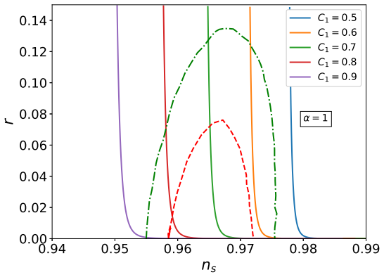
The argument is carried by warm-inflation slow-roll machinery specialized to the E-model. The dissipation ratio $Q=\Gamma/(3H)$ (here $\Gamma=C_1T$, linear in temperature) rescales the slow-roll conditions to $\varepsilon,\eta,\beta\ll 1+Q$ and enters the horizon-crossing power-spectrum amplitude through a thermal occupation factor and an enhancement function $G(Q_*)$ that models the growth of inflaton fluctuations from their coupling to the radiation bath. The load-bearing identity is the strong-regime reduction: from $\rho_r/V=\varepsilon Q/[2(1+Q)^2]$ and $T/H=3Q/C_1$, which follow from the radiation-production balance $4H\rho_r=\Gamma\dot\varphi^2$ and the slow-roll equation of motion, the amplitude collapses to a potential-independent form $\Delta_R=\frac{5C_1^3}{12g_*\pi^4Q_*^2}\bigl(1+\sqrt{3\pi Q_*}/\sqrt{3+4\pi Q_*}\bigr)G(Q_*)$ (Eq 58), with $g_*=228.75$. Differentiating $\ln\Delta_R$ through $n_s = 1+\frac{Q_*}{3+5Q_*}(6\varepsilon-2\eta)\frac{1}{\Delta_R}\frac{d\Delta_R}{dQ_*}$ (Eq 60) yields the spectral index, and $r=2V/(3\pi^2M_P^4\Delta_R)$ (Eqs 64–66) yields the tensor-to-scalar ratio; the two chosen enhancement functions, $G_1$ for plateau-like potentials and $G_2$ from warm little inflation, close the system and generate the $n_s$–$r$ trajectories compared with the Planck 2018 contours.
What would settle it
Take Eq 57, insert the explicit E-model potential, its strong-regime slow-roll parameter $\varepsilon$ (Eq 42), and the horizon-crossing $Q_*$ (Eq 47), and verify that the printed potential-independent amplitude (Eq 58) is reproduced across the $C_1$ windows of Tables 2 and 3; an independent numerical integration of the dissipative curvature-perturbation equations for the same potential settles the same question. As an observable cross-check, evaluate Eq 58 at those parameters and compare with the measured curvature amplitude $A_s\simeq2.1\times10^{-9}$, since the paper's contour plots test only the shape of the spectrum, not its absolute amplitude.
Extended reading notes
Core claim
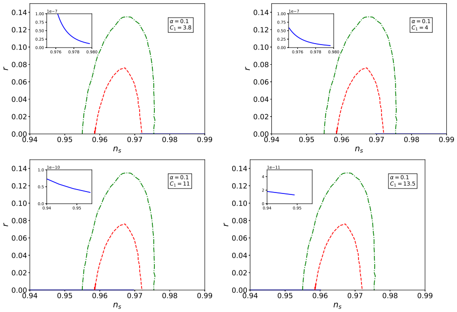
The central claim, stated by the authors, is that warm inflation preserves the E-model's observational status: with the potential $V(\varphi)=\lambda M_P^4\bigl(1-e^{-\sqrt{2/(3\alpha)}\,\varphi/M_P}\bigr)^2$ and dissipation $\Gamma=C_1T$, the slow-roll analysis yields closed-form observables in both regimes. In the weak regime ($Q\ll1$) the paper finds $n_s = 1 - \frac{9\alpha}{2N^2} - \frac{2}{N} + Q_*\bigl(\frac{6\alpha}{N^2}+\frac{4}{3N}\bigr)$ and $r = 12\alpha/N^2$, so that Planck 2018 imposes $C_1^4/\alpha \lesssim 1.6\times10^{-7}$, with upper bounds on $C_1$ for each $\alpha$ (for instance $C_1<0.04$ at $\alpha=1$). In the strong regime ($Q\gg1$) the scalar power spectrum reduces to a potential-independent expression in $C_1$ and $Q_*$ alone (Eq 58); the spectral index follows by differentiating it (Eq 63) and the tensor-to-scalar ratio from $r = 2V/(3\pi^2M_P^4\Delta_R)$ (Eq 66). With either enhancement function — the plateau-like $G_1$ or the warm-little-inflation $G_2$ — the predicted ($n_s$, $r$) trajectories stay inside the Planck 2018 contours for ranges of $C_1$ at each $\alpha$ in $10^{-2}<\alpha<10^4$, for example $3.8<C_1<13.5$ at $\alpha=0.1$ with $G_1$. The paper concludes that the warm $\alpha$-attractor E-model is observationally viable in both dissipative regimes.
Load-bearing premise
Everything the strong-regime analysis concludes rests on the claim that, at horizon crossing, the scalar-perturbation amplitude becomes independent of the potential's shape and reduces to a formula in only the dissipation coupling $C_1$ and the dissipation ratio $Q_*$, through two algebraic relations connecting radiation density, potential slope, and temperature; if those relations leave a hidden potential dependence, the printed $n_s$ and $r$ for the strong regime, and hence the claimed Planck compatibility, would have to be recomputed.
Editorial extensions
If this is right
- The warm $\alpha$-attractor E-model is compatible with Planck 2018 data in both weak and strong dissipation regimes, extending the model's observational viability from cold to warm inflation.
- Dissipation shifts the predicted ($n_s$, $r$) away from the cold-attractor values and opens parameter space that cold inflation leaves unexplored; the weak regime obeys $C_1^4/\alpha \lesssim 1.6\times10^{-7}$, and the strong regime admits windows such as $3.8<C_1<13.5$ for $\alpha=0.1$.
- The two physically motivated enhancement functions yield compatible but slightly different constraints, so the viability conclusion does not hinge on which microphysical picture of the dissipation is adopted.
- Because the paper's formulas connect $\alpha$, $C_1$, and the e-fold number $N$ directly to $n_s$ and $r$, any future tightening of the CMB bounds translates immediately into updated windows on the dissipation coupling.
Reading between the lines
- If the strong-regime analysis is right, its tensor-to-scalar ratio is extremely small — the plotted trajectories run at or below $r\sim10^{-7}$ for the shown parameters — so a future detection of primordial B-modes would effectively select the weak-regime branch of this model or rule the strong branch out.
- Equation 58 determines the scalar amplitude from $C_1$ and $Q_*$ alone, independent of $\alpha$; imposing the measured curvature amplitude $A_s\simeq2.1\times10^{-9}$ on that formula would fix the allowed $C_1$–$Q_*$ relation without any potential input, a normalization cross-check the paper does not run.
- The paper adopts a dissipation coefficient linear in temperature; repeating the derivation with $\Gamma\propto T^3$, or with a field-dependent coefficient, would show whether the Planck compatibility is special to this dissipation mechanism or generic to the warm E-model.
- The strong-regime $C_1$ windows narrow as $\alpha$ grows (from $3.8<C_1<13.5$ at $\alpha=0.1$ to $0.12<C_1<0.2$ at $\alpha=10$), suggesting the warm mechanism's parameter freedom concentrates near the small-$\alpha$ attractor end of the family.
Editorial analysis
A structured set of objections, weighed in public.
Referee Report
Summary. The paper studies warm inflation in the α-attractor E-model with a dissipation coefficient linear in temperature, Γ = C1 T. It derives slow-roll expressions for the scalar power spectrum, spectral index ns, and tensor-to-scalar ratio r in both the weak and strong dissipative regimes, and compares the resulting ns–r trajectories with Planck 2018 contours. The authors conclude that the warm E-model is observationally compatible with Planck in both regimes and that dissipation enlarges the viable parameter space.
Significance. If the central claim were established, the paper would provide useful analytic formulas for a specific, theoretically motivated warm-inflation model and a concrete comparison with CMB data. The authors make a genuine effort to derive closed-form expressions and to confront them with published Planck contours, which is a positive feature. However, the strong-regime comparison never imposes the observed scalar perturbation amplitude, and the weak-regime normalization is based on the cold-inflation COBE condition despite the thermal terms in the warm power spectrum. These issues are load-bearing for the paper's main claim of observational viability, and they need to be fixed before the conclusions can be trusted.
major comments (3)
- [§5.2, Eqs. (58), (63), (66) and Tables 2-3] The strong-regime analysis never imposes the observed scalar amplitude. Equation (58) expresses ΔR only through C1, Q*, and the enhancement function, and Eq. (49) determines Q* for specified α, C1, N, and λ. If λ is carried over from the weak-regime COBE condition, Eq. (34), the model makes a definite prediction for ΔR with no free overall scale. For a representative point shown in the figures, (α=0.1, C1=4, N=60), Eq. (58) with G1 gives ΔR ≈ 1.8×10^-4, about five orders of magnitude above the Planck-normalized value As ≈ 2.1×10^-9. The allowed intervals for C1 in Tables 2 and 3 therefore reflect only agreement with the ns–r contours and do not establish that the corresponding models produce the observed perturbation amplitude. The authors must redo the strong-regime constraints by imposing ΔR = As, which fixes λ (or the combination of parameters) for each α, C1, and N, and then recompute the predicted (ns, r) at that amplitude.
- [§4.1, Eqs. (32)-(34)] The weak-regime coupling λ is fixed by the cold-inflation COBE normalization V/ε = (0.0276 M_P)^4, Eq. (32), but the warm-inflation scalar power spectrum is given by Eq. (16), which contains thermal contributions involving n*, T*/H*, and G(Q*). Fixing λ with the cold normalization neglects these thermal effects; the correct procedure would be to impose the warm amplitude ΔR = As in the Q≪1 limit. Since λ enters Q* through Eq. (31) and hence enters ns through Eqs. (38)-(39), the weak-regime bounds on C1 in Table 1 and Fig. 1 are not self-consistent as they stand. The weak-regime analysis should be rederived using the warm amplitude normalization.
- [§4.2, Eq. (18)] The weak-regime temperature expression, Eq. (18), appears dimensionally inconsistent as printed. It gives T ∝ [C1 e^{-2x}/(α C* M_P^2 (1-e^{-x}))]^{1/3}, which has dimension [mass]^{-2/3} rather than energy. A factor λ^{1/2} M_P^3, or the equivalent after choosing units, is missing from the numerator. This error likely propagates into Eq. (30)-(31) for Q* and hence into the weak-regime expressions for ns. The authors should correct Eq. (18) and trace the consequences for the subsequent analytic results.
minor comments (3)
- [Table 3, α=1 row] The quoted allowed range '0.6 < C1 < 0.08' is internally contradictory, since the lower bound exceeds the upper bound. This appears to be a typographical error and should be corrected.
- [§5.1] The statement that Planck 2018 imposes an upper bound on C1^4/α of 1.6×10^-7 is not a direct output of the Planck data; it is a model-dependent bound obtained from the authors' ns–r trajectories. The wording should distinguish the observational contours used from the derived constraint.
- [General presentation] The paper contains several formulas whose rendering in the arXiv text is ambiguous or garbled, such as Eq. (30) and Eq. (50). The authors should ensure that the final typeset version displays all exponents and fractions unambiguously.
Circularity Check
No significant circularity; the C1 constraints are genuine parameter fits against Planck ns-r contours, and the external inputs (COBE normalization and the numerical G(Q) fits) do not encode the claimed predictions.
full rationale
The derivation chain is not circular. In the weak regime, lambda is fixed by the COBE normalization (Eqs. 32-34) to match the observed scalar amplitude, which is a standard calibration rather than a fit to ns or r; the subsequent ns-r trajectories (Eqs. 38-39) are genuine model predictions, with C1 later constrained by Planck contours. In the strong regime, the amplitude Eq. (58) is obtained algebraically from the preceding warm-inflation equations, and the enhancement functions G1 and G2 (Eqs. 53-54) are imported from independent numerical studies [66, 34], not calibrated to Planck data in this paper. The absence of an explicit scalar-amplitude normalization check in the strong regime is a correctness or benchmark gap, not a circular reduction: it does not make a fitted parameter masquerade as a prediction. No self-citation chain or uniqueness theorem is invoked, so the circularity score is zero.
Assumptions & free parameters
free parameters (5)
- α (α-attractor curvature parameter) =
scanned over 10^-2 to 10^4; constrained by Planck contours
- C1 (dissipation coefficient in Γ = C1 T) =
Tables 1-3, e.g., 3.8 < C1 < 13.5 for α=0.1 in the strong regime
- λ (E-model potential coupling) =
λ = (0.0276)^4 (3α)/(4N^2) from Eq 34
- N (number of e-folds at horizon exit) =
implied to be around 50-60, not specified per plot
- G1 and G2 fitting coefficients (0.18, 0.01, 0.335, 0.0185) =
as in Eqs 53 and 54
assumptions (6)
- domain assumption Steady-state radiation condition ˙ρr ≈ 0, so 4Hρr = Γ ˙φ² (Eq 11).
- domain assumption The perturbation spectrum Eq 16 with Bose-Einstein occupation n* ≈ T/H and enhancement functions G1/G2 from [34,66] applies to the E-model.
- domain assumption Thermal fluctuations dominate, so 1+2n* ≈ 2T/H = 6Q/C1 (Section 4.2).
- ad hoc to paper The cold-inflation COBE normalization V/ε = (0.0276 M_P)^4 fixes λ in the weak warm regime (Eqs 32-34).
- domain assumption Planck 2018 restricts α to 10^-2 < α < 10^4 (Section 5).
- domain assumption End of inflation occurs at ε = 1 in the weak regime and ε = Q in the strong regime (Eqs 24, 45-46).
Cite this review
Pith. "Pith review of The $\alpha$-Attractor E-Model in Warm Inflation: Observational Viability from Planck 2018." pith.science (2026). https://pith.science/paper/GPQ4VAEH
@misc{pith2026250606717,
  author       = {Pith},
  title        = {Pith review of: The $\alpha$-Attractor E-Model in Warm Inflation: Observational Viability from Planck 2018},
  year         = {2026},
  howpublished = {\url{https://pith.science/paper/GPQ4VAEH}},
  note         = {Machine review of arXiv:2506.06717}
}
abstract
We explore the inflationary evolution and observational viability of the $\alpha$-attractor E-model in the framework of warm inflation, focusing on both weak and strong dissipative regimes, with a dissipation coefficient linear in temperature. In the strong regime, we account for the growth of inflaton fluctuations due to coupling with the radiation bath via two different forms for the dissipation enhancement function: one associated with plateau-like potentials, and another motivated by the warm little inflation scenario. Employing slow roll conditions, we analytically derive the expressions for the key inflationary observables, the spectral index $n_s$ and the tensor-to-scalar ratio $r$, in both dissipative regimes. The resulting theoretical trajectories on the $n_s$--$r$ plane are then juxtaposed with the contour plots obtained from Planck 2018 data in order to constrain the model parameter. Our analysis shows that the warm $\alpha$-attractor E-model remains compatible with observations in both dissipative regimes, with dissipation playing a crucial role in shifting the predictions and enlarging the viable parameter space, highlighting observational robustness of the model when extended to warm inflation.
Figures


Figures from the paper (4 more)



Forward citations
Cited by 1 Pith paper
-
Behaviour of $\alpha$-attractors in Warm Inflation
In strongly dissipative warm inflation, T, E, and polynomial alpha-attractor models lose the cold-inflation attractor convergence in the n_s-r plane.
Reference graph
Works this paper leans on
-
[1]
Alan H. Guth. Inflationary universe: A possible solution to the hori- zon and flatness problems. Phys. Rev. D , 23:347–356, Jan 1981. URL: https://link.aps.org/doi/10.1103/PhysRevD.23.347, doi:10.1103/PhysRevD.23.347
-
[2]
Andrei D. Linde. A New Inflationary Universe Scenario: A P ossible Solution of the Horizon, Flatness, Homogeneity, Isotropy and Primordial Monopole P roblems. Phys. Lett. B , 108:389– 393, 1982. doi:10.1016/0370-2693(82)91219-9
-
[3]
K. Sato. First Order Phase Transition of a Vacuum and Expa nsion of the Universe. Mon. Not. Roy. Astron. Soc. , 195:467–479, 1981
1981
-
[4]
Andrei D. Linde. Chaotic Inflation. Phys. Lett. B , 129:177–181, 1983. doi:10.1016/0370-2693(83)90837-7
-
[5]
A D Linde. The inflationary universe. Rep. Prog. Phys. , 47(8):925, aug 1984. URL: https://dx.doi.org/10.1088/0034-4885/47/8/002, doi:10.1088/0034-4885/47/8/002
-
[6]
The inflationary universe
A.H.Guth and P.J.Steinhardt. The inflationary universe . Scientific American , 250:116–129,
-
[7]
Andreas Albrecht and Paul J. Steinhardt. Cosmology for g rand unified the- ories with radiatively induced symmetry breaking. Phys. Rev. Lett. , 48:1220– 1223, Apr 1982. URL: https://link.aps.org/doi/10.1103/PhysRevLett.48.1220, doi:10.1103/PhysRevLett.48.1220
-
[8]
Steinhardt, Michael S
Andreas Albrecht, Paul J. Steinhardt, Michael S. Turner , and Frank Wilczek. Reheating an inflationary universe. Phys. Rev. Lett. , 48:1437–1440, May
Show all 88 references
-
[10]
Larson et al
D. Larson et al. Seven-year wilkinson microwave anisot ropy probe (wmap) observations: Power spectra and wmap-derived parameters. Astrophys. J. Suppl. , 192:16, 2011. arXiv:1001.4635, doi:10.1088/0067-0049/192/2/16
2011 arXiv
-
[11]
C. L. Bennett et al. Seven-year wilkinson microwave ani sotropy probe (wmap) observations: Are there cosmic microwave background anomalies? Astrophys. J. Suppl. , 192:17, 2011. arXiv:1001.4758, doi:10.1088/0067-0049/192/2/17. 18
2011 arXiv
-
[12]
Jarosik et al
N. Jarosik et al. Seven-year wilkinson microwave aniso tropy probe (wmap) observa- tions: Sky maps, systematic errors, and basic results. Astrophys. J. Suppl. , 192:14, 2011. arXiv:1001.4744, doi:10.1088/0067-0049/192/2/14
2011 arXiv
-
[13]
Hinshaw et al
G. Hinshaw et al. Nine-year wilkinson microwave anisot ropy probe (wmap) observations: Cosmological parameter results. Astrophys. J. Suppl. , 208:19, 2013. arXiv:1212.5226, doi:10.1088/0067-0049/208/2/19
2013 arXiv
-
[14]
P. A. R. Ade, N. Aghanim, C. Armitage-Caplan, M. Arnaud, M. Ashdown, F. Atrio-Barandela, and et al. Planck 2013 results. xvi. cosmological parameter s. Astron. Astrophys. , 571:A16,
2013
-
[15]
P. A. R. Ade, N. Aghanim, M. Arnaud, M. Ashdown, J. Aumont , C. Baccigalupi, and et al. Planck 2015 results. XIII. Cosmological parameters. Astron. Astrophys., 594:A13, 2016. arXiv:1502.01589, doi:10.1051/0004-6361/201525830
2015 arXiv
-
[16]
A. A. Starobinsky. A new type of isotropic cosmological models without singularity. Phys. Lett. B , 91:99–102, 1980. doi:10.1016/0370-2693(80)90670-X
1980 doi
-
[17]
V. F. Mukhanov and G. V. Chibisov. Quantum fluctuations a nd a nonsingular universe. JETP Lett., 33:532–535, 1981. [Pisma Zh. Eksp. Teor. Fiz. 33, 549 (1981 )]
1981
-
[18]
S. W. Hawking. The development of irregularities in a si ngle bubble inflationary universe. Phys. Lett. B , 115:295, 1982. doi:10.1016/0370-2693(82)90373-2
1982 doi
-
[19]
Guth and So-Young Pi
Alan H. Guth and So-Young Pi. Fluctuations in the new infl ationary universe. Phys. Rev. Lett., 49:1110–1113, 1982. doi:10.1103/PhysRevLett.49.1110
1982 doi
-
[20]
Bardeen, Paul J
James M. Bardeen, Paul J. Steinhardt, and Michael S. Tur ner. Spontaneous cre- ation of almost scale-free density perturbations in an infla tionary universe. Phys. Rev. D, 28:679–693, Aug 1983. URL: https://link.aps.org/doi/10.1103/PhysRevD.28.679, doi:10.1103/PhysRevD.28.679
1983 doi
-
[21]
A. A. Starobinsky. Dynamics of phase transition in the n ew inflationary uni- verse scenario and generation of perturbations. Phys. Lett. B , 117:175–178, 1982. doi:10.1016/0370-2693(82)90541-X
1982 doi
-
[22]
Liddle, Paul Parsons, and John D
Andrew R. Liddle, Paul Parsons, and John D. Barrow. Form aliz- ing the slow-roll approximation in inflation. Phys. Rev. D , 50:7222–7232, Dec 1994. URL: https://link.aps.org/doi/10.1103/PhysRevD.50.7222, doi:10.1103/PhysRevD.50.7222
1994 doi
-
[23]
Liddle and David H
Andrew R. Liddle and David H. Lyth. Cosmological Inflation and Large-Scale Structure . Cambridge University Press, New York, 2000
2000
-
[24]
Kolb and Michael S
Edward W. Kolb and Michael S. Turner. The Early Universe , volume 69 of Frontiers in Physics. Addison-Wesley, Redwood City, CA, 1990
1990
-
[25]
Starobinsky
Lev Kofman, Andrei Linde, and Alexei A. Starobinsky. Re - heating after inflation. Phys. Rev. Lett. , 73:3195–3198, Dec
-
[26]
Lev A. Kofman. The Origin of matter in the universe: Rehe ating after inflation. 5 1996. arXiv:astro-ph/9605155
1996 arXiv
-
[27]
Partic le production in the new infla- tionary cosmology
Laurence F Abbott, Edward Farhi, and Mark B Wise. Partic le production in the new infla- tionary cosmology. Phys. Lett. B , 117(1-2):29–33, 1982
1982
-
[28]
Reheating in Inflationary Cosmology: Theory and Applic ations
Rouzbeh Allahverdi, Robert Brandenberger, Francis-Y an Cyr-Racine, and Anupam Mazum- dar. Reheating in Inflationary Cosmology: Theory and Applic ations. Ann. Rev. Nucl. Part. Sci., 60:27–51, 2010. arXiv:1001.2600, doi:10.1146/annurev.nucl.012809.104511
2010 arXiv
-
[29]
Amin, Mark P
Mustafa A. Amin, Mark P. Hertzberg, David I. Kaiser, and Johanna Karouby. Nonperturbative Dynamics Of Reheating After Inflation: A Review. Int. J. Mod. Phys. D , 24:1530003, 2014. arXiv:1410.3808, doi:10.1142/S0218271815300037
2014 arXiv
-
[30]
Warm inflation
Arjun Berera. Warm inflation. Phys. Rev. Lett. , 75:3218–3221, Oct
-
[31]
Arjun Berera and Rudnei O. Ramos. Affinity for scalar field s to dissipate. Phys. Rev. D, 63:103509, Apr 2001. URL: https://link.aps.org/doi/10.1103/PhysRevD.63.103509, doi:10.1103/PhysRevD.63.103509
2001 doi
-
[32]
The warm inflation story
Arjun Berera. The warm inflation story. Universe, 9(6), 2023. URL: https://www.mdpi.com/2218-1997/9/6/272, doi:10.3390/universe9060272
2023 doi
-
[33]
Warm inflation in the adiabatic regime — a m odel, an existence proof for inflationary dynamics in quantum field theory
Arjun Berera. Warm inflation in the adiabatic regime — a m odel, an existence proof for inflationary dynamics in quantum field theory. Nuclear Physics B , 585(3):666–714,
-
[34]
Ramos, and Jo˜ ao G
Mar Bastero-Gil, Arjun Berera, Rudnei O. Ramos, and Jo˜ ao G. Rosa. Warm little inflaton. Phys. Rev. Lett. , 117:151301, Oct
-
[35]
Warm-viscous inflation model on t he brane in light of planck data
V Kamali and M R Setare. Warm-viscous inflation model on t he brane in light of planck data. Classical and Quantum Gravity , 32(23):235005, nov 2015. URL: https://dx.doi.org/10.1088/0264-9381/32/23/235005, doi:10.1088/0264-9381/32/23/235005
2015 doi
-
[36]
M. R. Setare and V. Kamali. Warm chaplygin inflation in lo op quan- tum cosmology in light of planck data. Phys. Rev. D , 91:123517, Jun
-
[37]
Tac hyon warm-intermediate inflation in the light of planck data
Vahid Kamali, Spyros Basilakos, and Ahmad Mehrabi. Tac hyon warm-intermediate inflation in the light of planck data. Eur. Phys. J. C , 76(10):525, Sep 2016. doi:10.1140/epjc/s10052-016-4380-6
2016 doi
-
[38]
Observational constraints on monomia l warm infla- tion
Luca Visinelli. Observational constraints on monomia l warm infla- tion. Journal of Cosmology and Astroparticle Physics , 2016(07):054, jul 2016. URL: https://dx.doi.org/10.1088/1475-7516/2016/07/054, doi:10.1088/1475-7516/2016/07/054. 20
2016 doi
-
[39]
Warm-tachyo n gauss–bonnet infla- tion in the light of planck 2015 data
Meysam Motaharfar and Hamid Reza Sepangi. Warm-tachyo n gauss–bonnet infla- tion in the light of planck 2015 data. Eur. Phys. J. C , 76(11):646, Nov 2016. doi:10.1140/epjc/s10052-016-4474-1
2015 doi
-
[40]
Warm λ 4 φ4 inflationary universe model in light of planck 2015 results
Grigorios Panotopoulos and Nelson Videla. Warm λ 4 φ4 inflationary universe model in light of planck 2015 results. Eur. Phys. J. C , 75(11):525, Nov 2015. doi:10.1140/epjc/s10052-015-3764-3
2015 doi
-
[41]
Non-minimal higgs inflation in the contex t of warm scenario in the light of planck data
Vahid Kamali. Non-minimal higgs inflation in the contex t of warm scenario in the light of planck data. Eur. Phys. J. C , 78(11):975, Nov 2018. doi:10.1140/epjc/s10052-018-6449-x
2018 doi
-
[42]
Impact of generalized dissipative coefficient on warm inflationary dynamics in the l ight of latest planck data
Abdul Jawad, Shahzad Hussain, Shamaila Rani, and Nelso n Videla. Impact of generalized dissipative coefficient on warm inflationary dynamics in the l ight of latest planck data. Eur. Phys. J. C , 77(10):700, Oct 2017. doi:10.1140/epjc/s10052-017-5264-0
2017 doi
-
[43]
Dynamic s of warm power-law plateau in- flation with a generalized inflaton decay rate: predictions a nd constraints after planck 2015
Abdul Jawad, Nelson Videla, and Faiza Gulshan. Dynamic s of warm power-law plateau in- flation with a generalized inflaton decay rate: predictions a nd constraints after planck 2015. Eur. Phys. J. C , 77(5):271, Apr 2017. doi:10.1140/epjc/s10052-017-4846-1
2015 doi
-
[44]
War m intermediate inflation in the randall–sundrum ii model in the light of planck 2015 and bice p2 results: a general dissipative coefficient
Ram´ on Herrera, Nelson Videla, and Marco Olivares. War m intermediate inflation in the randall–sundrum ii model in the light of planck 2015 and bice p2 results: a general dissipative coefficient. Eur. Phys. J. C , 75(5):205, May 2015. doi:10.1140/epjc/s10052-015-3433-6
2015 doi
-
[45]
On warm natural inflation and planck 2018 constraints
Mahmoud AlHallak, Khalil Kalid Al-Said, Nidal Chamoun , and Moustafa Sayem El-Daher. On warm natural inflation and planck 2018 constraints. Universe, 9(2), 2023. URL: https://www.mdpi.com/2218-1997/9/2/80, doi:10.3390/universe9020080
2018 doi
-
[46]
Micol Benetti and Rudnei O. Ramos. Warm inflation dissip ative effects: Pre- dictions and constraints from the planck data. Phys. Rev. D , 95:023517, Jan 2017. URL: https://link.aps.org/doi/10.1103/PhysRevD.95.023517, doi:10.1103/PhysRevD.95.023517
2017 doi
-
[47]
Universality Class in Conformal Inflation
Renata Kallosh and Andrei Linde. Universality Class in Conformal Inflation. JCAP, 1307:002,
-
[48]
Universality classes of inflation
Diederik Roest. Universality classes of inflation. JCAP, 1401:007, 2014. arXiv:1309.1285, doi:10.1088/1475-7516/2014/01/007
2014 arXiv
-
[49]
Ramos, and Jo˜ ao G
Mar Bastero-Gil, Arjun Berera, Rudnei O. Ramos, and Jo˜ ao G. Rosa. General dissipation co- efficient in low-temperature warm inflation. Journal of Cosmology and Astroparticle Physics , 2013(01):016, jan 2013. URL: https://dx.doi.org/10.1088/1475-7516/2013/01/016, doi:10.1088/147...
2013 doi
-
[50]
Warm inflation with a general form of the dissip ative co- efficient
Yi Zhang. Warm inflation with a general form of the dissip ative co- efficient. Journal of Cosmology and Astroparticle Physics , 2009(03):023, mar 2009. URL: https://dx.doi.org/10.1088/1475-7516/2009/03/023, doi:10.1088/1475-7516/2009/03/023
2009 doi
-
[51]
Akrami et al
Y. Akrami et al. Planck 2018 results. X. Constraints on i nflation. Astron. Astrophys., 641:A10,
2018
-
[52]
P. A. R. Ade et al. Improved constraints on primordial gr avitational waves using planck, wmap, and bicep/keck observations through the 2018 observing sea son. Phys. Rev. Lett. , 127:151301, Oct 2021. URL: https://link.aps.org/doi/10.1103/PhysRevLett.127.151301, doi:10.1103/Ph...
2018 doi
-
[53]
Supe rconformal inflationary α-attractors
Renata Kallosh, Andrei Linde, and Diederik Roest. Supe rconformal inflationary α-attractors. JHEP, 11:198, 2013. arXiv:1311.0472, doi:10.1007/JHEP11(2013)198
2013 arXiv
-
[54]
Observational viab ility of an inflation model with e-model nonminimal derivative coupling
Kourosh Nozari and Narges Rashidi. Observational viab ility of an inflation model with e-model nonminimal derivative coupling. The Astrophysical Journal , 863(2), 2018. doi:10.3847/1538-4357/aad18e
2018 doi
-
[55]
Salamate, H
F. Salamate, H. Sheikhahmadi, and K. Saaidi. E-model α -attractor on brane from planck data and reheating temperature. Journal of Experimental and Theoretical Physics , 129:774– 780, 2019. doi:10.3103/S0027134919050114
2019 doi
-
[56]
Superconformal gener alizations of the starobin- sky model
Renata Kallosh and Andrei Linde. Superconformal gener alizations of the starobin- sky model. Journal of Cosmology and Astroparticle Physics , 2013(06):028, 2013. URL: https://iopscience.iop.org/article/10.1088/1475-751 6/2013/06/028, doi:10.1088/1475-7516/2013/06/028
2013 doi
-
[57]
Unity of Cos- mological Inflation Attractors
Mario Galante, Renata Kallosh, Andrei Linde, and Diede rik Roest. Unity of Cos- mological Inflation Attractors. Phys. Rev. Lett. , 114:141302, 2015. arXiv:1412.3797, doi:10.1103/PhysRevLett.114.141302
2015 arXiv
-
[58]
Planck, LHC, and α-attractors
Renata Kallosh and Andrei Linde. Planck, LHC, and α-attractors. Phys. Rev. D , 91(8):083528,
-
[59]
I.G. Moss. Primordial inflation with spontaneous symme - try breaking. Phys. Lett. B , 154(2):120–124, 1985. URL: https://www.sciencedirect.com/science/article/pii/0370269385905702, doi:https://doi.org/10.1016/0370-2693(85)90570-2
1985
-
[60]
Thermal properties of an inflationary uni verse
Arjun Berera. Thermal properties of an inflationary uni verse. Phys. Rev. D , 54:2519–2534, Aug 1996. URL: https://link.aps.org/doi/10.1103/PhysRevD.54.2519, doi:10.1103/PhysRevD.54.2519
1996 doi
-
[61]
Thermally induced densit y pertur- bations in the inflation era
Arjun Berera and Li-Zhi Fang. Thermally induced densit y pertur- bations in the inflation era. Phys. Rev. Lett. , 74:1912–1915, Mar
1912
-
[62]
A. Berera. Interpolating the Stage of Inflationary Univ erse: From Slow-roll to Warm Inflation. Phys. Rev. D , 54:2519–2534, 1996. arXiv:hep-th/9601134, doi:10.1103/PhysRevD.54.2519
1996 arXiv
-
[63]
A. Berera. Warm Inflation at Arbitrary Adiabaticity: A M odel, an Existence Proof for Inflationary Dynamics in Quantum Field Theory. Nucl. Phys. B , 585:666–714, 2000. arXiv:hep-ph/9904409, doi:10.1016/S0550-3213(00)00411-9
-
[64]
Lisa M. H. Hall, Ian G. Moss, and Arjun Berera. Scalar per tur- bation spectra from warm inflation. Phys. Rev. D , 69:083525, Apr
-
[65]
On the consistency of warm infla - tion
Ian G Moss and Chun Xiong. On the consistency of warm infla - tion. Journal of Cosmology and Astroparticle Physics , 2008(11):023, nov 2008. URL: https://dx.doi.org/10.1088/1475-7516/2008/11/023, doi:10.1088/1475-7516/2008/11/023. 22
2008 doi
-
[66]
Mar Bastero-Gil, Arjun Berera, Rafael Hern´ andez-Jim ´ enez, and Jo˜ ao G. Rosa. Dynam- ical and observational constraints on the warm little inflat on scenario. Phys. Rev. D , 98:083502, Oct 2018. URL: https://link.aps.org/doi/10.1103/PhysRevD.98.083502, doi:10.1103/PhysRevD....
2018 doi
-
[67]
Chris Graham and Ian G. Moss. Density fluctuations from w arm inflation. JCAP, 0907:013,
-
[68]
Warm inflation model b uilding
Mar Bastero-Gil and Arjun Berera. Warm inflation model b uilding. Int. J. Mod. Phys. A , 24:2207–2240, 2009. arXiv:0902.0521, doi:10.1142/S0217751X09044206
2009 arXiv
-
[69]
arXiv:1502.07733, doi:10.1103/PhysRevD.91.083528
-
[70]
A. N. Taylor and Arjun Berera. Perturbation spectra in t he warm inflationary scenario. Phys. Rev. D , 62:083517, 2000. arXiv:astro-ph/0006077, doi:10.1103/PhysRevD.62.083517
2000 arXiv
-
[71]
H. P. de Oliveira and S. E. Joras. On perturbations in war m inflation. Phys. Rev. D , 64:063513,
-
[72]
Bezrukov, D
F. Bezrukov, D. Gorbunov, and M. Shaposhnikov. On initi al condi- tions for the hot big bang. J. Cosmol. Astropart. Phys. , 2009(06):029, jun 2009. URL: https://dx.doi.org/10.1088/1475-7516/2009/06/029, doi:10.1088/1475-7516/2009/06/029
2009 doi
-
[73]
URL: https://link.aps.org/doi/10.1103/PhysRevLett.74.1912, doi:10.1103/PhysRevLett.74.1912
1912 doi
-
[74]
Planck 2018 results- VI
N Aghanim, Y Akrami, M Ashdown, J Aumont, C Baccigalupi, M Ballardini, A.J Banday, R.B Barreiro, N Bartolo, S Basak, et al. Planck 2018 results- VI. Cosmological parameters. Astron. Astrophys., 641:A6, 2020. 23
2018
-
[83]
Ramos and L
Rudnei O. Ramos and L. A. da Silva. Power spectrum for infl ation models with quantum and thermal noises. JCAP, 1303:032, 2013. arXiv:1302.3544, doi:10.1088/1475-7516/2013/03/032
2013 arXiv
-
[88]
Warm inflation model b uilding
Mar Bastero-Gil and Arjun Berera. Warm inflation model b uilding. Int. J. Mod. Phys. A , 24(12):2207–2240, 2009. arXiv:https://doi.org/10.1142/S0217751X09044206, doi:10.1142/S0217751X09044206
2009 doi
-
[1982]
URL: https://link.aps.org/doi/10.1103/PhysRevLett.48.1437, doi:10.1103/PhysRevLett.48.1437
-
[1984]
URL: http://www.jstor.org/stable/24969372
-
[1994]
URL: https://link.aps.org/doi/10.1103/PhysRevLett.73.3195, doi:10.1103/PhysRevLett.73.3195. 19
-
[1995]
URL: https://link.aps.org/doi/10.1103/PhysRevLett.75.3218, doi:10.1103/PhysRevLett.75.3218
-
[2000]
URL: https://www.sciencedirect.com/science/article/pii/S0550321300004119, doi:https://doi.org/10.1016/S0550-3213(00)00411-9
-
[2001]
arXiv:gr-qc/0103089, doi:10.1103/PhysRevD.64.063513
-
[2004]
URL: https://link.aps.org/doi/10.1103/PhysRevD.69.083525, doi:10.1103/PhysRevD.69.083525
-
[2009]
arXiv:0905.3500, doi:10.1088/1475-7516/2009/07/013
2009 arXiv
-
[2013]
arXiv:1306.5220, doi:10.1088/1475-7516/2013/07/002
2013 arXiv
-
[2014]
arXiv:1303.5076, doi:10.1051/0004-6361/201321591
-
[2015]
URL: https://link.aps.org/doi/10.1103/PhysRevD.91.123517, doi:10.1103/PhysRevD.91.123517
-
[2016]
URL: https://link.aps.org/doi/10.1103/PhysRevLett.117.151301, doi:10.1103/PhysRevLett.117.151301
-
[2020]
arXiv:1807.06211, doi:10.1051/0004-6361/201833887
Reviewed August 7, 2026 · model on record in the stance chip above.
Discussion (0). Continue with ORCID to comment.