REVIEW 3 major objections 5 minor 44 references
Post-processing subtraction of tilt-to-length noise in LISA in the presence of gravitational wave signals
T0 review · 3 major / 5 minor · reviewed 2026-08-12 · deepseek-v4-flash
Pith's one-line read Gravitational-wave contamination doesn't break LISA's tilt-to-length noise subtraction.
desk verdict Solid engineering validation for LISA TTL subtraction with GW signals; abstract overstates signal-preservation evidence. read the letter →
The pith
A machine-rendered reading of the paper's core claim, the machinery that carries it, and where it could break.
The reading
What carries the argument
The load-bearing object is the linear tilt-to-length coupling model of Eq. (3), $\hat{x}^{\mathrm{TTL}}_{ij} = C^{\varphi\mathrm{Rx}}_{ij}\varphi^{\mathrm{DWS}}_{ij} + C^{\eta\mathrm{Rx}}_{ij}\eta^{\mathrm{DWS}}_{ij} + \cdots$: each of the six links has four coupling coefficients multiplying the differential-wavefront-sensing measured angular jitter of the local and remote spacecraft/MOSA pairs, with the remote terms delayed by the light travel time. Propagated through second-generation time-delay interferometry into the orthogonal AET combinations, this model becomes the template that the Markov-chain Monte Carlo fitter matches to the simulated length data, iteratively whitening the noise between 3 mHz and 0.9 Hz; the fitted coefficients then define the subtraction. The argument's strength rests on this linear template being the true coupling and on the fit band being populated by white jitter.
What would settle it
Run the same one-day MCMC fit on simulated LISA data in which the spacecraft/MOSA jitter follows a colored spectrum, such as the control-loop roll-off expected in flight, with a massive black hole merger overlapping the fit band; the central claim fails if coefficient errors exceed 0.1 mm/rad or if the residual after subtracting the fitted TTL model no longer matches the injected GW waveform.
Extended reading notes
Core claim
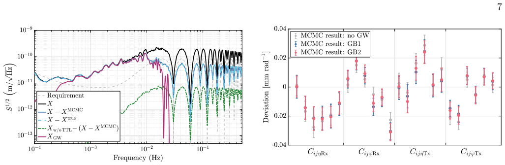
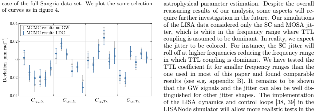
The central claim is that the post-processing TTL subtraction scheme planned for LISA works essentially as well when gravitational-wave signals are present as when they are absent. Using simulated one-day data with identical noise and jitter realizations, the authors fit the 24 TTL coupling coefficients of the linear model (Eq. 3) to TDI AET data with an iterative-whitening Markov-chain Monte Carlo algorithm over the 3 mHz–0.9 Hz band. For verification binaries, a stochastic gravitational-wave background, detached galactic white dwarf binaries, massive black hole binary mergers, and the combined multi-source data set, estimated coefficient deviations stay below the 0.1 mm/rad requirement, residuals after subtraction lie below the LISA mission noise requirement, and the residual TTL noise remains about an order of magnitude below the other instrument noises. Comparing the fitted-TTL-subtraction residual with the injected GW response in data that contain no other instrument noise shows that the subtraction does not perceivably alter the GW signal. The authors also show that changing arm lengths, whether from Keplerian or ESA science orbits, do not change the conclusions, supporting the static-arm assumption of earlier work.
Load-bearing premise
The load-bearing premise is that the true TTL coupling is exactly the linear model of Eq. (3) with white spacecraft and MOSA jitter in the 3 mHz–0.9 Hz fit band; if real jitter is colored or the coupling has unmodeled nonlinearity or slow drifts, the fitted coefficients and subtraction residuals could degrade beyond the reported margins.
Editorial extensions
If this is right
- The planned post-processing TTL subtraction can be run on LISA data without first separating or masking gravitational-wave signals; the tested source classes and the combined multi-source data set all leave coefficient errors below 0.1 mm/rad.
- After subtraction the total noise meets the LISA requirement even when a massive black hole merger overlaps the TTL-dominated band, so the noise cleanup does not have to wait for quiet data stretches.
- Because the GW response in the residuals matches the injected signal, the subtraction does not imprint a spurious waveform component, which is a prerequisite for unbiased astrophysical parameter estimation.
- The static-unequal-arm assumption used in earlier TTL subtraction studies is adequate: Keplerian and ESA science orbit arm-length changes give nearly identical residuals.
- The combined multi-source data set behaves like the merger-dominated case, indicating that the loudest source on a given day controls the TTL fit quality.
Reading between the lines
- If real spacecraft/MOSA jitter is colored rather than white, the effective TTL-dominated band shrinks and the fit leans on low frequencies where GW confusion is strongest; testing the same MCMC scheme with control-loop-shaped jitter would show whether the 0.1 mm/rad margin survives.
- The one-day analysis leaves open long-integration effects: over months of data, slow drifts of coupling coefficients or a slowly evolving GW foreground could bias the TTL fit, so the claim should be re-checked on full-mission-length simulations with parameter-estimation follow-up.
- The linear model in Eq. (3) omits possible nonlinear or time-varying TTL terms; a dedicated injection of a nonlinear coupling term would reveal how much unmodeled structure the fit absorbs into the linear coefficients.
- Extending to source classes not tested here, such as extreme-mass-ratio inspirals or a cosmological stochastic background, would stress the low-frequency band where the GW response sits above the TTL noise; the paper itself identifies these as open cases.
Editorial analysis
A structured set of objections, weighed in public.
Referee Report
Summary. The paper investigates whether post-processing subtraction of tilt-to-length (TTL) noise in LISA remains accurate and non-destructive when gravitational wave (GW) signals are present in the data. The authors simulate one day of LISA data with LISANode, include four classes of GW signals (verification binaries, a stochastic GW background, galactic white-dwarf binaries, massive black hole binary mergers, and a full LDC Sangria combination), and use an MCMC fit to estimate the 24 TTL coupling coefficients in the TDI AET variables. They report that coefficient estimation errors remain below the 0.1 mm/rad requirement, that residual noise after subtraction stays below the LISA requirement, and that visual overlays of amplitude spectral densities suggest the GW signal is not degraded by the subtraction. The manuscript also confirms that static-arm simulations are adequate despite small real arm-length variations.
Significance. If the central claim holds, the paper provides valuable evidence for the LISA data-processing pipeline: TTL noise subtraction should not be catastrophically confused with GW signals, and the subtraction itself should not corrupt the GW response. The study's strengths include the use of realistic LISANode simulations, public LDC data, multiple GW source types, and an MCMC estimator that is not given the true coupling coefficients, so the coefficient-error results are a genuine test of the estimation procedure. The residual ASDs and coefficient-error plots are informative and support the main quantitative claims about noise subtraction. However, the claim that 'GW signal characteristics were not altered' is supported only by qualitative ASD overlays over one day of data, which is not sufficient for the strength of the abstract statement.
major comments (3)
- [Section V.C, V.D and Summary] The abstract's claim that 'the GW signal characteristics were not altered by the TTL coupling subtraction' is not supported by the evidence presented. In Fig. 9 and Fig. 14 the test is a visual overlap between the ASD of the injected GW response (purple) and the residual obtained by subtracting the fitted TTL model from data with no instrument noise other than TTL (yellow). An ASD match is insensitive to phase-coherent distortions, time shifts, or spectral leakage, any of which could bias astrophysical parameter recovery while leaving the ASD nearly unchanged. The Summary itself concedes that the signal-preservation point 'was shown only indirectly in figures 9 and 14 for one day of data' and that confirmation with longer integration times and parameter estimation is required. Please either add a phase-coherent or parameter-estimation test on the residual data, or qualify the abstract and conclusions accordingly.
- [Abstract and Section V.D] The simulations assume jitter that is white in the 3 mHz to 0.9 Hz fit band (Appendix A, Eqs. (A1)-(A3)), while real LISA jitter is expected to be colored. Section V.D states: 'We cannot say, whether or how other jitter shapes would affect the findings of this paper.' Because the central claim concerns in-flight applicability, this is a substantial limitation. The abstract should not present the results without this caveat. Either demonstrate robustness to a colored-jitter model (e.g., by repeating the coefficient-fit and subtraction tests with a roll-off or otherwise colored spectrum) or explicitly scope the headline claim to the white-jitter case.
- [Section V.C, V.D and Summary] All signal-preservation tests are performed on one day of data. The claim that GW signals are not altered is therefore limited to a one-day timescale; the Summary acknowledges that longer integration times and the ultimate effect on astrophysical parameter estimation remain open. Since LISA science analyses will integrate for weeks to months, the manuscript should either extend the analysis to a longer data stretch or at least move the one-day limitation into the abstract so that the strength of the claim matches the evidence.
minor comments (5)
- [Section II heading] The heading 'TIL T-TO-LENGTH NOISE IN LISA' contains a typo; it should read 'TILT-TO-LENGTH NOISE IN LISA'.
- [Appendix A] In the sentence introducing the interferometer noises, 'lenght readout' should be 'length readout'.
- [Figure 2 caption] The caption spells 'Keplarian' orbits; the standard spelling is 'Keplerian'.
- [Section V.A] The verification binary 'HMCnc' is presumably 'HM Cnc' (the cataclysmic variable HM Cancri); please use the standard astronomical designation.
- [Section V.D] The phrase 'The here presented results cannot directly be compared with [10]' would read more naturally as 'The results presented here cannot be directly compared with [10]'.
Circularity Check
No circularity: the GW-robustness claim is tested with an MCMC estimator that is not given the true TTL coefficients or the injected GW signals, and the same-model simulation limits scope without making the result definitional.
full rationale
The paper's central empirical claim is that an MCMC estimator of the 24 TTL coupling coefficients, applied to simulated TDI-AET data containing injected GW signals, still estimates the coefficients to within 0.1 mm/rad and that subtraction leaves the GW response essentially unchanged. This is not a circular derivation: the GW signals come from external simulators (LISANode, LISA GW Response, and the Sangria/LDC data sets), and the estimator is not given the true coupling coefficients or the GW waveforms. Equation (3) is the assumed physical noise model used to construct the simulated TTL noise; it is not a quantity the paper claims to derive from the data. The subtraction checks are direct consistency checks: after subtracting the fitted model, the residual is compared with the injected GW response (Figs. 9 and 14), so the result could have failed if the GW signals biased the coefficient estimates. The paper itself limits the strength of the signal-preservation claim: 'the latter was shown only indirectly in figures 9 and 14 for one day of data. The results would need to be confirmed considering the longer integration times for GW analyses and their ultimate effect on the astrophysical parameter estimation.' It also explicitly flags the white-jitter scope limitation: 'We cannot say, whether or how other jitter shapes would affect the findings of this paper.' These are validation limitations, not circular steps. The self-citations to [7] and [8] for the fitting scheme are standard method attribution; they do not supply the GW-robustness result, which is tested against independent simulated benchmarks in this paper. No fitted parameter is renamed as a prediction, and no load-bearing uniqueness claim is imported from the authors' prior work. Therefore no step reduces by construction to its input; the appropriate circularity score is 0.
Assumptions & free parameters
free parameters (4)
- True TTL coupling coefficient C =
2.3 mm/rad
- Fit frequency range =
3 mHz to 0.9 Hz
- Jitter amplitudes =
SC 5 nrad/√Hz, MOSA 2 and 1 nrad/√Hz
- DWS readout noise =
70/335 nrad/√Hz
assumptions (5)
- domain assumption TTL coupling is linear in angles at nanoradian jitter (Eq. 3)
- domain assumption Jitter and instrument noise spectra in Appendix A represent LISA
- standard math The MCMC estimator from [7] converges and is unbiased under the simulated model
- domain assumption TDI AET combinations are suitable for fitting with no cross-correlation
- domain assumption Static unequal arm lengths are sufficient for TTL studies
Cite this review
Pith. "Pith review of Post-processing subtraction of tilt-to-length noise in LISA in the presence of gravitational wave signals." pith.science (2026). https://pith.science/paper/GTCFANGH
@misc{pith2026241114191,
  author       = {Pith},
  title        = {Pith review of: Post-processing subtraction of tilt-to-length noise in LISA in the presence of gravitational wave signals},
  year         = {2026},
  howpublished = {\url{https://pith.science/paper/GTCFANGH}},
  note         = {Machine review of arXiv:2411.14191}
}
read the original abstract
The Laser Interferometer Space Antenna (LISA) will be the first space-based gravitational wave (GW) observatory. It will measure gravitational wave signals in the frequency regime from 0.1 mHz to 1 Hz. The success of these measurements will depend on the suppression of the various instrument noises. One important noise source in LISA will be tilt-to-length (TTL) coupling. Here, it is understood as the coupling of angular jitter, predominantly from the spacecraft, into the interferometric length readout. The current plan is to subtract this noise in-flight in post-processing as part of a noise minimization strategy. It is crucial to distinguish TTL coupling well from the GW signals in the same readout to ensure that the noise will be properly modeled. Furthermore, it is important that the subtraction of TTL noise will not degrade the GW signals. In the present manuscript, we show on simulated LISA data and for four different GW signal types that the GW responses have little effect on the quality of the TTL coupling fit and subtraction. Also, the GW signal characteristics were not altered by the TTL coupling subtraction.
Figures


Figures from the paper (11 more)





Reference graph
Works this paper leans on
-
[1]
static arms with beam propagation times: τ12 ≈ 8.425 s, τ13 ≈ 8.322 s, τ23 ≈ 8.372 s, τ21 ≈ 8.322 s, τ31 ≈ 8.322 s, τ32 ≈ 8.372 s
-
[2]
changing arm lengths gained from Keplerian orbit files [25]
-
[3]
The static arm lengths given are those assumed in [7]
changing arm lengths gained from ESA LISA sci- ence orbit files [25, 26]. The static arm lengths given are those assumed in [7]. While the lengths for the individual links are within the LISA length variations, the variations for the full con- stellation were chosen for study purposes and may not be particularly realistic. We find larger arm length vari- ...
-
[4]
M-S Hartig, S Schuster, G Heinzel, and G Wanner. Non- geometric tilt-to-length coupling in space interferometry: mechanisms and analytical descriptions. Journal of Op- tics, 25(5):055601, apr 2023
work page 2023
-
[5]
LISA: unveiling a hidden universe
K Danzmann, T Prince, P Binetruy, P Bender, S Buch- man, J Centrella, M Cerdonio, N Cornish, M Cruise, C Cutler, et al. LISA: unveiling a hidden universe. As- sessment Study Report ESA/SRE, 3:2, 2011
work page 2011
-
[6]
M Colpi, K Danzmann, M Hewitson, K Holley- Bockelmann, P Jetzer, G Nelemans, A Petiteau, D Shoe- maker, C Sopuerta, R Stebbins, et al. LISA definition study report. ArXiv e-prints, 2024
work page 2024
-
[7]
M-S Hartig, S Schuster, and G Wanner. Geometric tilt- to-length coupling in precision interferometry: mecha- nisms and analytical descriptions. Journal of Optics, 24(6):065601, 2022
work page 2022
-
[8]
S. Paczkowski et al. Update on TTL coefficient estima- tion for LISA using noise minimisation, 2024. In prepa- ration
work page 2024
Show all 44 references
-
[9]
Preliminary results on the suppression of sensing cross-talk in LISA Pathfinder
G Wanner, N Karnesis, and LISA Pathfinder collabora- tion. Preliminary results on the suppression of sensing cross-talk in LISA Pathfinder. Journal of Physics: Con- ference Series, 840(1):012043, 2017
2017
-
[10]
Armano, H
M. Armano, H. Audley, J. Baird, M. Born, D. Bortoluzzi, N. Cardines, E. Castelli, A. Cavalleri, A. Cesarini, A. M. Cruise, et al. Tilt-to-length coupling in LISA Pathfinder: A data analysis. Phys. Rev. D, 108:102003, Nov 2023
2023
-
[11]
Paczkowski, R
S. Paczkowski, R. Giusteri, M. Hewitson, N. Karnesis, E. D. Fitzsimons, G. Wanner, and G. Heinzel. Postpro- cessing subtraction of tilt-to-length noise in LISA. Phys. Rev. D, 106:042005, Aug 2022
2022
-
[12]
Houba, S
N. Houba, S. Delchambre, T. Ziegler, G. Hechenblaikner, and W. Fichter. LISA spacecraft maneuver design to estimate tilt-to-length noise during gravitational wave events. Phys. Rev. D, 106:022004, Jul 2022
2022
-
[13]
George, J
D. George, J. Sanjuan, P. Fulda, and G. Mueller. Calcu- lating the precision of tilt-to-length coupling estimation and noise subtraction in LISA using Fisher information. Phys. Rev. D, 107:022005, Jan 2023
2023
-
[14]
Hartig, J
M-S. Hartig, J. Marmor, D. George, S. Paczkowski, and J. Sanjaun. Tilt-to-length coupling in LISA – uncertainty and biases. ArXiv e-prints, 2024
2024
-
[15]
Houba, S
N. Houba, S. Delchambre, T. Ziegler, and W. Fichter. Optimal estimation of tilt-to-length noise for spaceborne gravitational-wave observatories. J. Guid. Control Dyn., 45(6):1078–1092, 2022
2022
-
[16]
Time-delay interferometry
M Tinto and S Dhurandhar. Time-delay interferometry. Living Rev. Relativ., 24(1), 2021
2021
-
[17]
Wegener, S
H. Wegener, S. Paczkowski, M-S. Hartig, M. Hewitson, G. Heinzel, and G. Wanner. Design of dedicated tilt-to- length calibration maneuvers for LISA. ArXiv e-prints, 2024
2024
-
[18]
Auto- matic alignment of optical interferometers
E Morrison, B Meers, D Robertson, and H Ward. Auto- matic alignment of optical interferometers. Appl. Opt., 33(22), 1994
1994
-
[19]
Methods for simulat- ing the readout of lengths and angles in laser interfer- ometers with Gaussian beams
G Wanner, G Heinzel, E Kochkina, C Mahrdt, B Sheard, S Schuster, and K Danzmann. Methods for simulat- ing the readout of lengths and angles in laser interfer- ometers with Gaussian beams. Optics communications, 285(24):4831–4839, 2012
2012
-
[20]
Uncovering gravitational-wave backgrounds from noises of unknown shape with LISA
Q Baghi, N Karnesis, J-B Bayle, M Besan¸ con, and H In- chausp´ e. Uncovering gravitational-wave backgrounds from noises of unknown shape with LISA. J. Cosmol. Astropart. Phys, 2023(04):066, apr 2023
2023
-
[21]
Second- generation time-delay interferometry
M Tinto, S Dhurandhar, and D Malakar. Second- generation time-delay interferometry. Phys. Rev. D, 107:082001, Apr 2023
2023
-
[22]
Wanner, S
G. Wanner, S. Shah, M. Staab, H. Wegener, and S. Paczkowski. In-depth modeling of tilt-to-length cou- pling in LISA’s interferometers and TDI Michelson ob- servables. Phys. Rev. D, 110:022003, Jul 2024
2024
-
[23]
LISA optimal sensitivity
T A Prince, M Tinto, S L Larson, and J W Armstrong. LISA optimal sensitivity. Phys. Rev. D, 66:122002, Dec 2002
2002
-
[24]
PyTDI (1.3.1)
M Staab, J-B Bayle, and O Hartwig. PyTDI (1.3.1). Zen- odo, 2023. https://doi.org/10.5281/zenodo.8429119
2023 doi
-
[25]
Technical Report No
M Hewitson. Technical Report No. LISA-LCST-INST- DD-003. Max-Planck Institute for Gravitational Physics (Albert Einstein Institute), 2021
2021
-
[26]
LISANode (1.4)
J-B Bayle, O Hartwig, A Petiteau, and M Lilley. LISANode (1.4). Zenodo, September 2022. https: //doi.org/10.5281/zenodo.6461078
2022 doi
-
[27]
Optical Simulations
to generate the LISA data sets and considered ESA LISA science orbits [26]. In the other cases we used the ‘Sangria’ data set from the LISA Data Challenge (LDC) 2a [28, 29]. As these data sets were created for equal arm length orbits, we simulated an orbit file with these prop...
-
[28]
Unified model for the LISA measurements and instrument simulations
J-B Bayle and O Hartwig. Unified model for the LISA measurements and instrument simulations. Phys. Rev. 11 D, 107:083019, Apr 2023
2023
-
[29]
LISA Orbits (2.3)
J-B Bayle, A Hees, M Lilley, C Le Poncin-Lafitte, W Martens, and E Joffre. LISA Orbits (2.3). Zenodo,
-
[30]
LISA Con- stants (1.3)
J-B Bayle, M Le Jeune, and A Hees. LISA Con- stants (1.3). Zenodo, 2022. https://doi.org/10.5281/ zenodo.6627346
2022
-
[31]
Trajectory design for the ESA LISA mission
W Martens and E Joffre. Trajectory design for the ESA LISA mission. J. Astronaut. Sci., 68, Jun 2021
2021
-
[32]
LISA GW Response (1.1)
J-B Bayle, Q Baghi, A Renzini, and M Le Jeune. LISA GW Response (1.1). Zenodo, 2022. https://doi.org/ 10.5281/zenodo.6423436
2022 doi
-
[33]
LISA Data Challenge San- gria (LDC2a) (Version v2) [Data set]
M Le Jeune and S Babak. LISA Data Challenge San- gria (LDC2a) (Version v2) [Data set]. Zenodo, 2022. https://doi.org/10.5281/zenodo.7132178
2022 doi
-
[34]
LISA Data Chal- lenge software (1.2.0)
LISA Data Challenge working group. LISA Data Chal- lenge software (1.2.0). Zenodo, 2022. https://doi.org/ 10.5281/zenodo.7332221
2022 doi
-
[35]
Cosmology with the laser interferometer space antenna
P Auclair, D Bacon, T Baker, T Barreiro, N Bartolo, E Belgacem, N Bellomo, I Ben-Dayan, D Bertacca, M Be- sancon, et al. Cosmology with the laser interferometer space antenna. Living Rev. Relativ., 26(5), Aug 2023
2023
-
[36]
LISA galactic binaries with astrometry from Gaia DR3
T Kupfer, V Korol, T B Littenberg, S Shah, E Savalle, P J Groot, T R Marsh, M Le Jeune, G Nelemans, A F Pala, A Petiteau, G Ramsay, D Steeghs, and S Babak. LISA galactic binaries with astrometry from Gaia DR3. Astrophys. J., 963(2):100, mar 2024
2024
-
[37]
Abbott, T
R. Abbott, T. D. Abbott, S. Abraham, F. Acernese, K. Ackley, A. Adams, C. Adams, R. X. Adhikari, V. B. Adya, C. Affeldt, et al. Upper limits on the isotropic gravitational-wave background from Advanced LIGO and Advanced Virgo’s third observing run. Phys. Rev. D, 104:022004, Jul 2021
2021
-
[38]
Impact of the noise knowledge uncertainty for the science exploitation of cos- mological and astrophysical stochastic gravitational wave background with LISA
M Muratore, J Gair, and L Speri. Impact of the noise knowledge uncertainty for the science exploitation of cos- mological and astrophysical stochastic gravitational wave background with LISA. Phys. Rev. D, 109:042001, Feb 2024
2024
-
[39]
Stochastic gravitational wave background reconstruction for a nonequilateral and unequal-noise LISA constella- tion
O Hartwig, M Lilley, M Muratore, and M Pieroni. Stochastic gravitational wave background reconstruction for a nonequilateral and unequal-noise LISA constella- tion. Phys. Rev. D, 107:123531, Jun 2023
2023
-
[41]
Stochastic gravitational wave background from stellar origin binary black holes in LISA
S Babak, C Caprini, D G Figueroa, N Karnesis, P Mar- coccia, G Nardini, M Pieroni, A Ricciardone, A Sesana, and J Torrado. Stochastic gravitational wave background from stellar origin binary black holes in LISA. Journal of Cosmology and Astroparticle Physics, 2023(08):034, aug 2023
2023
-
[42]
LISA Data Challenge: Sangria
S Babak, M Le Jeune, A Petiteau, and M Val- lisneri. LISA Data Challenge: Sangria. Ref.-No. LISA-LCST-SGS-MAN-001, 2021. https://lisa- ldc.lal.in2p3.fr/static/data/pdf/LDC-manual- Sangria.pdf
2021
-
[43]
New LISA dynamics feedback control scheme: Common-mode isolation of test mass control and probes of test-mass acceleration
H Inchausp´ e, M Hewitson, O Sauter, and P Wass. New LISA dynamics feedback control scheme: Common-mode isolation of test mass control and probes of test-mass acceleration. Phys. Rev. D, 106:022006, Jul 2022
2022
-
[44]
LISA dynamics and control: Closed-loop simulation and numerical demonstration of time delay interferometry
L Heisenberg, H Inchausp´ e, D Q Nam, O Sauter, R Waibel, and P Wass. LISA dynamics and control: Closed-loop simulation and numerical demonstration of time delay interferometry. Phys. Rev. D, 108:122007, Dec 2023. Appendix A: Jitters and noises used in our analysis In this sec...
2023
-
[2023]
https://doi.org/10.5281/zenodo.7700361
Reviewed August 12, 2026 · model on record in the stance chip above.
Discussion (0). Continue with ORCID to comment.