REVIEW 3 major objections 4 minor 82 references
Trend Filtering -- I. A Modern Statistical Tool for Time-Domain Astronomy and Astronomical Spectroscopy
T0 review · 3 major / 4 minor · reviewed 2026-08-14 · deepseek-v4-flash
Pith's one-line read Trend filtering is minimax optimal for spatially heterogeneous signals and beats every linear smoother.
desk verdict A solid, honest methods-transfer paper that would land better if the abstract matched the theorem: trend filtering is minimax-optimal over L1 Sobolev classes, not universally superior to linear smoothers. read the letter →
The pith
A machine-rendered reading of the paper's core claim, the machinery that carries it, and where it could break.
The reading
What carries the argument
The central object is the trend filtering estimator, defined as the solution to $\min_{m} \sum_i (f(t_i)-m(t_i))^2 w_i + \gamma \sum_i |\Delta^{(k+1)} m(t_i)| \Delta t$, where $\Delta^{(k+1)}$ is the discrete $(k+1)$-st derivative; this is an L1 analog of the smoothing spline problem and an $\ell^1$ relaxation of variable-knot regression splines. Equivalently, in the falling factorial basis it is a lasso with a single tuning parameter $\gamma$. The $\ell^1$ penalty drives most knot coefficients to zero, giving automatic knot selection and local adaptivity, while the generalized lasso structure (identity predictor, banded penalty) permits an ADMM algorithm with near-linear practical complexity. The hyperparameter is selected by Stein's unbiased risk estimate for fixed-input error or 10-fold cross-validation for random-input error, using the exact degrees of freedom formula $\mathrm{df}(\hat{f}_0)=E[\text{number of knots}]+k+1$.
What would settle it
Simulate worst-case mean-squared error over a well-specified L1 Sobolev ball of heterogeneous signals, comparing trend filtering against the best linear smoother tuned with oracle knowledge of the signal; if any linear smoother matches trend filtering's $n^{-2/3}$ rate for $k=0$, the paper's central optimality claim is false.
Extended reading notes
Core claim
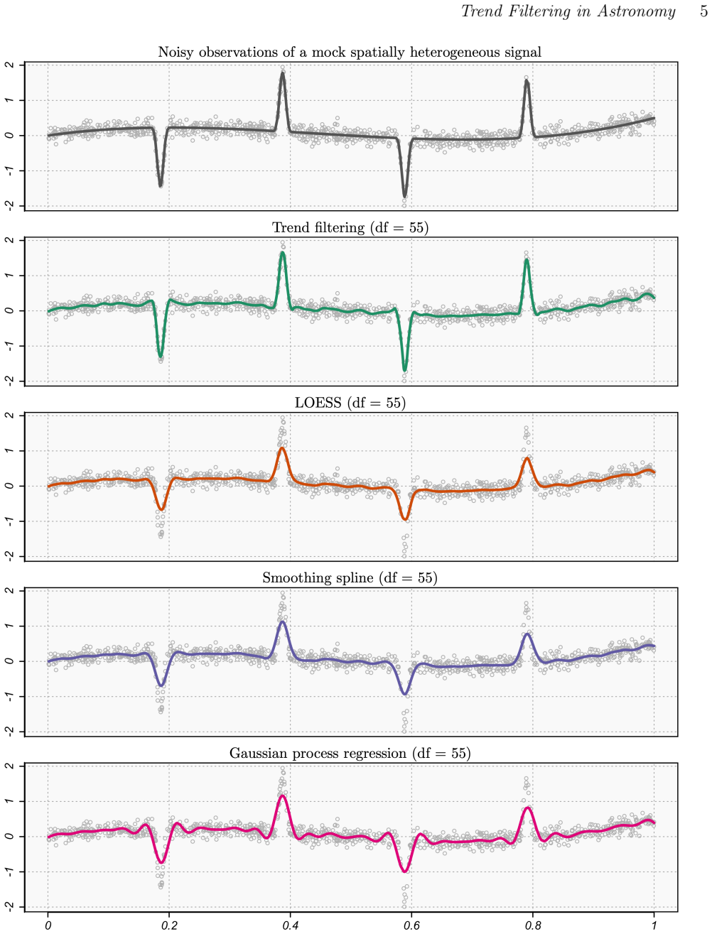
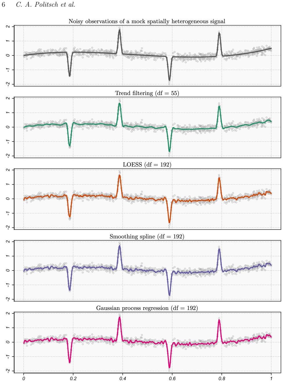
The central claim is that trend filtering simultaneously meets four requirements no classical method meets: statistical optimality for spatially heterogeneous signals, practical analysis assumptions (unequally spaced inputs, heteroskedastic noise), scalable computation, and a one-dimensional hyperparameter space with automatic selection. The estimator fits a kth-order piecewise polynomial with knots chosen automatically by an $\ell^1$ penalty on discrete $(k+1)$-st derivatives, i.e. a total-variation penalized least squares problem. The paper's theoretical case relies on results that linear smoothers are uniformly suboptimal over L1 Sobolev classes, while trend filtering attains the minimax rate, e.g. $n^{-2/3}$ for $k=0$ versus at best $n^{-1/2}$ for linear smoothers. The empirical comparison fixes all methods at 55 effective degrees of freedom and shows trend filtering recovering both the smooth trend and sharp localized features, whereas LOESS, smoothing splines, and Gaussian process regression oversmooth the features; the linear smoothers need 192 degrees of freedom to match, and then overfit elsewhere.
Load-bearing premise
The central superiority claim is guaranteed only for signals belonging to an L1 Sobolev class, which the paper equates with 'spatially heterogeneous' signals; if real light curves and spectra fall outside that class, the minimax theorem does not ensure trend filtering beats linear smoothers in practice.
Editorial extensions
If this is right
- Denoising light curves with trend filtering should recover transient events such as supernova rises and exoplanet transits without the oversmoothing and ringing that fixed-bandwidth linear smoothers produce.
- Spectroscopic continuum and line flux estimates can be obtained in one fit, since the estimator separates smooth continuum from localized absorption and emission features while accounting for heteroskedastic per-pixel noise.
- Survey-scale data sets ($n \gtrsim 10^7$) can be processed within minutes on a single machine, making the method practical for current and upcoming large surveys.
- Users get a single hyperparameter, selected automatically, instead of Gaussian-process kernel parameters or locally varying bandwidths, removing a major source of manual tuning.
- The minimax rate gap implies a sample-equivalence result: for $k=0$ heterogeneous signals, a linear smoother needs about $n^{4/3}$ observations to learn as fast as trend filtering, so trend filtering is especially valuable in low-signal or sparse regimes.
Reading between the lines
- The same two-stage relaxation idea used here—select knots with an $\ell^1$ penalty, then refit by weighted least squares—could be applied to other $\ell^1$-penalized estimators in astronomy to reduce shrinkage bias while keeping automatic knot selection.
- If real astronomical signals deviate from L1 Sobolev classes, for instance by being fractal or containing multi-scale noise, the minimax guarantee is not directly binding; a natural extension is to test trend filtering against wavelet denoising on unequally sampled real data, where wavelet optimality is void.
- Because trend filtering is nonlinear, its sampling distribution is non-Gaussian even for Gaussian noise; the paper's bootstrap recommendations imply that reporting only Gaussian error bars for denoised light curves will understate uncertainty, and quantile bands should be adopted widely.
- The $n^{4/3}$ sample-size equivalence could inform survey design: to detect sharp spectral features at a given significance with linear methods one needs substantially more exposure time, whereas with trend filtering shorter exposures may suffice.
Signed reviews
Editorial analysis
A structured set of objections, weighed in public.
Referee Report
Summary. This paper introduces trend filtering to the astronomical community as a locally adaptive nonparametric denoiser for one-dimensional signals with spatially varying smoothness. The authors argue in Section 2 that linear smoothers are suboptimal for such signals, citing minimax results of Nemirovskii et al. and Tibshirani, and present a simulation comparing trend filtering with LOESS, smoothing splines, and Gaussian process regression at fixed effective degrees of freedom. Section 3 provides a tutorial-style description of trend filtering, its relationship to splines, software, hyperparameter selection via SURE and cross-validation, bootstrap uncertainty quantification, and a relaxed variant. The paper's concrete contributions are the astronomical exposition, the SURE selection recipe, three bootstrap algorithms, and supplementary R code.
Significance. If the claims are taken with appropriate qualifications, the paper addresses a genuine need: many astronomical time series and spectra combine smooth continua with sharp features, and standard linear smoothers are not locally adaptive. Trend filtering is a principled alternative with a minimax optimality guarantee over L1 Sobolev classes, flexible sampling requirements, a single tuning parameter, and scalable algorithms. The paper also ships code and clear recipes. However, the manuscript currently overstates the practical meaning of the minimax results and does not quantitatively demonstrate the finite-sample advantage it claims; these are fixable within the scope of the paper.
major comments (3)
- [Abstract; Section 2.1.2] The abstract's claim that 'when the underlying signal is spatially heterogeneous, trend filtering is superior to any statistical estimator that is a linear combination of the observed data' is stated without qualification. The supporting theory in Section 2.1.2 is a minimax result over the L1 Sobolev class F1,k in Eq. (14): trend filtering achieves the optimal worst-case rate, while linear smoothers do not. This is a worst-case, asymptotic statement over a specific function class, not a guarantee of lower error for every heterogeneous signal. The manuscript itself says the definition of 'spatially heterogeneous' is 'intentionally mathematically imprecise' and notes that L1 Sobolev classes contain spatially homogeneous signals as well, so the abstract overstates the theorem. Please rephrase the abstract to say 'minimax optimal over L1 Sobolev classes (signals with derivatives of bounded variation)' and treat the representativeness of real astronomical signals as a stated, testable premise.
- [Section 2.2; Figures 1 and 2] The empirical comparison is visual only. The text reports that trend filtering with 55 effective degrees of freedom is sufficient while LOESS, smoothing splines, and Gaussian process regression require 192 to recover the localized features, but no quantitative error metric (e.g., mean squared prediction error) is reported, no averaging over independent noise realizations is shown, and no uncertainty is attached to the comparison. This single hand-constructed signal is offered as evidence of 'clear practical consequences' for the theoretical gap. The argument would be much stronger with a table of error metrics computed over repeated simulations and, ideally, over several signal shapes.
- [Section 3.2; Abstract] The scalability claim that trend filtering handles n ≳ 10^7 within a few minutes appears in the abstract and in Section 3.2, but it is a summary of Ramdas and Tibshirani (2016) and is not reproduced or benchmarked here. Because practical scalability is one of the paper's advertised properties (P3 in Section 1), either provide a small timing benchmark in this paper or explicitly mark the abstract statement as a claim from the cited literature.
minor comments (4)
- [Section 4] The text refers to 'Table 3.4' for software links, but the table in Section 3.4 is numbered Table 2; please correct the cross-reference.
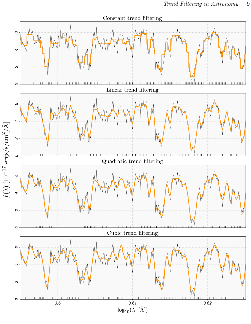
- [Figure 3 caption] The caption says the constant trend filtering estimate is discontinuous at the knots but is 'interpolate[d] here for visual purposes'; this should be clarified in the main text so that readers do not mistake the plotted curve for the actual piecewise-constant estimator.
- [Table 1] The binomial coefficient in the variable-knot regression splines row is printed as n!/(n!(n−p)!) but should be n!/(p!(n−p)!).
- [Equation (16)] The radial basis functions φ_j in the simulation are not specified; please state their exact form, width, and location so the simulation is reproducible.
Circularity Check
No significant circularity: the central claims are inherited from external minimax theory rather than derived from fitted inputs or self-citations.
full rationale
The paper's central superiority claim is not derived from its own fitted values. Section 2.1.2 explicitly attributes the minimax suboptimality of linear smoothers on L1 Sobolev classes to Nemirovskii et al. (1985) and Nemirovskii (1985), and attributes trend filtering's minimax optimality to Tibshirani (2014); the scalability claim is attributed to Ramdas and Tibshirani (2016). These are external, parameter-free mathematical results with stated assumptions, not results whose premises include the paper's conclusions. The paper's original additions (SURE hyperparameter selection, bootstrap variability bands, and relaxed trend filtering) are presented as methodology and are not used to establish the abstract's optimality claim. The definition of 'spatially heterogeneous' is admittedly imprecise and is connected to L1 Sobolev classes only as a commonly considered class; no equation defines the term in terms of trend filtering's minimax rate, so the abstract's claim is not tautologically forced by the paper's own definitions. The only self-references (Paper II and Wasserman's textbooks) are expositional and non-load-bearing. No fitted parameter is renamed as a prediction, and no self-citation chain is invoked to forbid alternatives.
Assumptions & free parameters
free parameters (1)
- Effective degrees of freedom in simulation comparison =
55
assumptions (4)
- domain assumption L1 Sobolev classes are the right model for spatially heterogeneous astronomical signals.
- standard math Trend filtering achieves the minimax rate over L1 Sobolev classes (Tibshirani 2014) and linear smoothers do not (Nemirovskii et al. 1985).
- standard math The effective degrees of freedom formula for trend filtering equals expected number of knots plus k+1 (Tibshirani and Taylor 2012), used in SURE.
- standard math The ADMM algorithm of Ramdas and Tibshirani (2016) solves trend filtering in O(n^1.5) worst case and near O(n) in practice.
Cite this review
Pith. "Pith review of Trend Filtering -- I. A Modern Statistical Tool for Time-Domain Astronomy and Astronomical Spectroscopy." pith.science (2026). https://pith.science/paper/H2LYTSEE
@misc{pith2026190807151,
  author       = {Pith},
  title        = {Pith review of: Trend Filtering -- I. A Modern Statistical Tool for Time-Domain Astronomy and Astronomical Spectroscopy},
  year         = {2026},
  howpublished = {\url{https://pith.science/paper/H2LYTSEE}},
  note         = {Machine review of arXiv:1908.07151}
}
abstract
The problem of denoising a one-dimensional signal possessing varying degrees of smoothness is ubiquitous in time-domain astronomy and astronomical spectroscopy. For example, in the time domain, an astronomical object may exhibit a smoothly varying intensity that is occasionally interrupted by abrupt dips or spikes. Likewise, in the spectroscopic setting, a noiseless spectrum typically contains intervals of relative smoothness mixed with localized higher frequency components such as emission peaks and absorption lines. In this work, we present trend filtering, a modern nonparametric statistical tool that yields significant improvements in this broad problem space of denoising $spatially$ $heterogeneous$ signals. When the underlying signal is spatially heterogeneous, trend filtering is superior to any statistical estimator that is a linear combination of the observed data---including kernel smoothers, LOESS, smoothing splines, Gaussian process regression, and many other popular methods. Furthermore, the trend filtering estimate can be computed with practical and scalable efficiency via a specialized convex optimization algorithm, e.g. handling sample sizes of $n\gtrsim10^7$ within a few minutes. In a companion paper, we explicitly demonstrate the broad utility of trend filtering to observational astronomy by carrying out a diverse set of spectroscopic and time-domain analyses.
Figures
Reference graph
Works this paper leans on
-
[1]
Aigrain S., Parviainen H., Pope B. J. S., 2016, MNRAS, 459, 2408
2016
-
[2]
B., Tibshirani R
Arnold T. B., Tibshirani R. J., 2016, Journal of Computational and Graphical Statistics, 25, 1
2016
-
[3]
B., Sadhanala V., Tibshirani R
Arnold T. B., Sadhanala V., Tibshirani R. J., 2014, Fast algorithms for generalized lasso problems , https://github.com/glmgen
work page 2014
- [4]
- [5]
-
[6]
G., 1952, The Annals of Mathematical Statistics, 23, 315
Cochran W. G., 1952, The Annals of Mathematical Statistics, 23, 315
work page 1952
-
[7]
Contreras C., et al., 2010, AJ, 139, 519
work page 2010
-
[8]
Croft R. A. C., et al., 2002, ApJ, 581
work page 2002
Show all 82 references
-
[9]
pp 12--20
De Boor C., 1974, in Conference on the numerical solution of differential equations. pp 12--20
1974
-
[10]
De Boor C., 1978, in Applied Mathematical Sciences
1978
-
[11]
Dhawan S., Leibundgut B., Spyromilio J., Maguire K., 2015, MNRAS, 448, 1345
2015
-
[12]
Diamond S., Boyd S., 2016, Journal of Machine Learning Research, 17, 1
2016
-
[13]
R., Kass R
Dimatteo I., Genovese C. R., Kass R. E., 2001, Biometrika, 88, 1055
2001
-
[14]
Dimitriadis G., et al., 2017, MNRAS, 468, 3798
2017
-
[15]
L., Johnstone I
Donoho D. L., Johnstone I. M., 1994, Probability Theory and Related Fields, 99, 277
1994
-
[16]
L., Johnstone I
Donoho D. L., Johnstone I. M., 1998, The Annals of Statistics, 26, 879
1998
-
[17]
Efron B., 1979, The Annals of Statistics, 7, 1
1979
-
[18]
Efron B., 1986, Journal of the American Statistical Association, 81, 461
1986
-
[19]
Efron B., Tibshirani R., 1986, Statistical Science, 1, 54
1986
-
[20]
Fan J., 1993, The Annals of Statistics, 21, 196
1993
-
[21]
Fan J., Gijbels I., 1992, The Annals of Statistics, 20, 2008
1992
-
[22]
Series B (Methodological), 57, 371
Fan J., Gijbels I., 1995, Journal of the Royal Statistical Society. Series B (Methodological), 57, 371
1995
-
[23]
Fan J., Gasser T., Gijbels I., Brockmann M., Engel J., 1997, Annals of the Institute of Statistical Mathematics, 49, 79
1997
-
[24]
R., Minin V
Faulkner J. R., Minin V. N., 2018, Bayesian Analysis, 13, 225
2018
-
[25]
Figueiredo M. A. T., 2003, IEEE Transactions on Pattern Analysis and Machine Intelligence, 25, 1150
2003
-
[26]
K., 1997, A&AS, 124, 579
Fligge M., Solanki S. K., 1997, A&AS, 124, 579
1997
-
[27]
P., Aigrain S., Roberts S., Evans T
Gibson N. P., Aigrain S., Roberts S., Evans T. M., Osborne M., Pont F., 2012, MNRAS, 419, 2683
2012
-
[28]
Gijbels I., Mammen E., 1998, Scandinavian Journal of Statistics, 25, 503
1998
-
[29]
Z., Butler N
Golkhou V. Z., Butler N. R., 2014, ApJ, 787, 90
2014
-
[30]
G \' o mez-Valent A., Amendola L., 2018, JCAP, 2018, 051
2018
-
[31]
Gy \"o rfi L., Kohler M., Krzyzak A., Walk H., 2002, in Springer Series in Statistics
2002
-
[32]
B., et al., 2002, ApJS, 141
Hall P. B., et al., 2002, ApJS, 141
2002
-
[33]
Springer
Hastie T., Tibshirani R., Friedman J., 2009, The Elements of Statistical Learning: Data Mining, Inference and Prediction, 2 edn. Springer
2009
-
[34]
A., et al., 2005, ApJ, 634, 1190
Howell D. A., et al., 2005, ApJ, 634, 1190
2005
-
[35]
A., Hasminiskii R
Ibragimov I. A., Hasminiskii R. Z., 1980, Zapiski Nauchnykh Seminarov LOMI (in Russian), 97, 88
1980
-
[36]
L., 1978, SIAM Journal on Numerical Analysis, 15, 328
Jupp D. L., 1978, SIAM Journal on Numerical Analysis, 15, 328
1978
-
[37]
Kim S.-J., et al., 2009, SIAM Review, 51, 339
2009
-
[38]
Koh K., Kim S.-J., Boyd S., 2008, l1\_tf : Software for l1 Trend Filtering , http://stanford.edu/ boyd/l1_tf/
2008
-
[39]
Kornblith S., 2014, Lasso/Elastic Net linear and generalized linear models, https://github.com/JuliaStats/Lasso.jl
2014
-
[40]
W., 2005, MNRAS, 356, 557
Kov \'a cs G., Bakos G., Noyes R. W., 2005, MNRAS, 356, 557
2005
-
[41]
R., 1989, The Annals of Statistics, 17, 1217
Kunsch H. R., 1989, The Annals of Statistics, 17, 1217
1989
-
[42]
Department of Statistics, Stanford University
Land S., Friedman J., 1996, Technical report, Variable fusion: a new method of adaptive signal regression. Department of Statistics, Stanford University
1996
-
[43]
V., Mammen E., Spokoiny V
Lepski O. V., Mammen E., Spokoiny V. G., 1997, The Annals of Statistics, 25, 929
1997
-
[44]
Liu R., 1988, The Annals of Statistics, 16, 1696
1988
-
[45]
Mammen E., 1993, The Annals of Statistics, 21, 255
1993
-
[46]
L., Howes G
Maron J. L., Howes G. G., 2003, ApJ, 595, 564
2003
-
[47]
Meinshausen N., 2007, Computational Statistics & Data Analysis, 52, 374
2007
-
[48]
Muller H.-G., Stadtmuller U., 1987, The Annals of Statistics, 15, 610
1987
-
[49]
Nemirovskii A., 1985, Izv. Akad. Nauk. SSSR Tekhn. Kibernet. (in Russian), 3, 50
1985
-
[50]
Nemirovskii A., Polyak B., Tsybakov A., 1985, Problems of Information Transmission, 21
1985
-
[51]
Nussbaum M., 1985, The Annals of Statistics, 13, 984
1985
-
[52]
J., Schervish M
Paciorek C. J., Schervish M. J., 2004, in Advances in neural information processing systems. pp 273--280
2004
-
[53]
J., Schervish M
Paciorek C. J., Schervish M. J., 2006, Environmetrics, 17, 483
2006
-
[54]
Park T., Casella G., 2008, Journal of the American Statistical Association, 103, 681
2008
-
[55]
Pearson K., 1900, The London, Edinburgh, and Dublin Philosophical Magazine and Journal of Science, 50, 157
1900
-
[56]
V., Verde L., 2010, Phys
Peiris H. V., Verde L., 2010, Phys. Rev., D81, 021302
2010
-
[57]
E., Madore B
Persson S. E., Madore B. F., Krzemi \'n ski W., Freedman W. L., Roth M., Murphy D. C., 2004, AJ, 128, 2239
2004
-
[58]
A., Cisewski-Kehe J., Croft R
Politsch C. A., Cisewski-Kehe J., Croft R. A. C., Wasserman L., 2020, MNRAS, 492
2020
-
[59]
J., 2016, Journal of Computational and Graphical Statistics, 25, 839
Ramdas A., Tibshirani R. J., 2016, Journal of Computational and Graphical Statistics, 25, 839
2016
-
[60]
I., Osher S., Faterni E., 1992, Physica D: Nonlinear Phenomena, 60, 259
Rudin L. I., Osher S., Faterni E., 1992, Physica D: Nonlinear Phenomena, 60, 259
1992
-
[61]
M., O'Hagan A., 2003, Journal of the Royal Statistical Society
Schmidt A. M., O'Hagan A., 2003, Journal of the Royal Statistical Society. Series B (Statistical Methodology), 65, 743
2003
-
[62]
Steidl G., Didas S., Neumann J., 2006, International Journal of Computer Vision, 70, 241
2006
-
[63]
M., 1981, The Annals of Statistics, 9, 1135
Stein C. M., 1981, The Annals of Statistics, 9, 1135
1981
-
[64]
J., 1982, The Annals of Statistics, 10, 1040
Stone C. J., 1982, The Annals of Statistics, 10, 1040
1982
-
[65]
Tennyson J., 2019, Astronomical Spectroscopy: an Introduction to the Atomic and Molecular Physics of Astronomical Spectroscopy
2019
-
[66]
Theuns T., Zaroubi S., 2000, MNRAS, 317, 989
2000
-
[67]
Series B (Methodological), 58, 267
Tibshirani R., 1996, Journal of the Royal Statistical Society. Series B (Methodological), 58, 267
1996
-
[68]
J., 2014, The Annals of Statistics, 42, 285
Tibshirani R. J., 2014, The Annals of Statistics, 42, 285
2014
-
[69]
J., 2015, Statistica Sinica, pp 1265--1296
Tibshirani R. J., 2015, Statistica Sinica, pp 1265--1296
2015
-
[70]
J., Taylor J., 2011, The Annals of Statistics, 39, 1335
Tibshirani R. J., Taylor J., 2011, The Annals of Statistics, 39, 1335
2011
-
[71]
J., Taylor J., 2012, The Annals of Statistics, 40, 1198
Tibshirani R. J., Taylor J., 2012, The Annals of Statistics, 40, 1198
2012
-
[72]
Tibshirani R., Saunders M., Rosset S., Zhu J., Knight K., 2005, Journal of the Royal Statistical Society: Series B, 67, 91
2005
-
[73]
Tolstov A., Nomoto K., Sorokina E., Blinnikov S., Tominaga N., Taniguchi Y., 2019, ApJ, 881, 35
2019
-
[74]
B., 2008, Introduction to Nonparametric Estimation, 1st edn
Tsybakov A. B., 2008, Introduction to Nonparametric Estimation, 1st edn. Springer Publishing Company, Incorporated
2008
-
[75]
W., 1998, Asymptotic Statistics
Van der Vaart A. W., 1998, Asymptotic Statistics. Cambridge Series in Statistical and Probabilistic Mathematics, Cambridge University Press
1998
-
[76]
CBMS-NSF Regional Conference Series in Applied Mathematics, Society for Industrial and Applied Mathematics
Wahba G., 1990, Spline Models for Observational Data. CBMS-NSF Regional Conference Series in Applied Mathematics, Society for Industrial and Applied Mathematics
1990
-
[77]
P., Jebara T., eds, Proceedings of Machine Learning Research Vol
Wang Y.-X., Smola A., Tibshirani R., 2014, in Xing E. P., Jebara T., eds, Proceedings of Machine Learning Research Vol. 32, Proceedings of the 31st International Conference on Machine Learning. PMLR, Bejing, China, pp 730--738
2014
-
[78]
Wang Y.-X., et al., 2016, Journal of Machine Learning Research, 17, 1
2016
-
[79]
Springer Publishing Company, Incorporated
Wasserman L., 2003, All of Statistics: A Concise Course in Statistical Inference. Springer Publishing Company, Incorporated
2003
-
[80]
Springer Texts in Statistics
Wasserman L., 2006, All of Nonparametric Statistics. Springer Texts in Statistics
2006
-
[81]
E., Kasen D., Blinnikov S., Sorokina E., 2007, ApJ, 662, 487
Woosley S. E., Kasen D., Blinnikov S., Sorokina E., 2007, ApJ, 662, 487
2007
-
[82]
Wu C., 1986, The Annals of Statistics, 14, 1261
1986
Reviewed August 14, 2026 · model on record in the stance chip above.
Discussion (0). Continue with ORCID to comment.