OMGPT: A Sequence Modeling Framework for Data-driven Operational Decision Making

Guanting Chen; Hanzhao Wang; Kalyan Talluri; Xiaocheng Li

REVIEW 3 major objections 6 minor 1 cited by

OMGPT: A Sequence Modeling Framework for Data-driven Operational Decision Making

T0 review · 3 major / 6 minor · reviewed 2026-08-15 · deepseek-v4-flash

Challenge this review Re-run · record.json Download PDF Read on arXiv ↗ Review JSON

Pith's one-line read A single transformer pretrained on generated optimal-action sequences can act as a near-optimal decision algorithm for dynamic pricing, inventory, queueing, and revenue management without assuming an analytical model.

desk verdict Real and potentially useful pretraining scheme for OR decision making, but the sub-linear regret theorem leans on an assumed exploration structure that the paper never derives. read the letter →

arxiv 2505.13580 v1 pith:H46YXYHI submitted 2025-05-19 cs.LG cs.AI

Hanzhao Wang , Guanting Chen , Kalyan Talluri , Xiaocheng Li This is my paper · ORCID

classification cs.LGcs.AI

keywords sequencemodelinggenerativepre-trainedtransformeroperationaldecisionmakingdynamicpricingnewsvendorproblemqueueingcontrolrevenuemanagementBayesian

verification ladder T0 review T1 audit T2 compute T3 formal

The pith

A machine-rendered reading of the paper's core claim, the machinery that carries it, and where it could break.

The reading

This paper tries to establish that sequential operational decisions—what price to set, how much inventory to order, how fast to serve a queue, which requests to accept—can be solved as one sequence-prediction problem. It builds a GPT model, OMGPT, pretrains it on generated histories labelled with the optimal action at each step, and then deploys the same network as the decision algorithm, without assuming any demand or cost model. The paper claims OMGPT consistently outperforms problem-specific benchmark algorithms across all four tasks, generalizes to longer horizons and shifted environment distributions, and handles non-stationary or mixed demand types. If this holds, prior knowledge becomes easy to inject through pretraining data, and supervised learning becomes a route to decision algorithms that discover policies rather than imitate known ones.

What carries the argument

The central object is the optimal-action sequence prediction reformulation. An algorithm f is treated as a sequence function from any history H_t to an action a_t; the paper chooses f from the family of GPT-style transformer networks TF_theta by minimizing the empirical prediction loss against the optimal action a*_t on histories sampled from a prior distribution over environments. The load-bearing identity is the Bayes-optimal function Alg*(H) = argmin_a E_gamma[ l(a, a*_t) | H ], the action minimizing expected loss with respect to the posterior over environments. The theory treats TF_hat_theta as Alg* plus a small deviation, with a reward-gap constant Delta_Exploit and an information-gain constant Delta_Explore controlling the regret bound, while the architecture interleaves feature embeddings of contexts and observations with action embeddings and uses a context window to extend beyond the pretraining horizon.

What would settle it

Measure, on held-out environments from the prior, the actual reward gap E[r(X_t, Alg*(H_t)) - r(X_t, TF_hat_theta(H_t)) | H_t] and the KL divergence between observation distributions induced by nearby environment parameters at each history. If the gap grows with t, or the KL information per unit parameter distance vanishes for any plausible history, Theorem 5.9's sub-linear bound does not apply and the empirical success would need a different explanation.

Watch

Extended reading notes

Core claim

On the paper's own terms, the central discovery is that predicting the optimal action from the history is enough to drive near-optimal decisions across a broad class of operations problems, even though the underlying environment is unknown. The pretrained transformer TF_hat_theta is analyzed as a Bayes-optimal decision function Alg* that minimizes expected prediction loss under the prior over environments; depending on the loss, Alg* behaves as posterior sampling, posterior averaging, or posterior median. The paper argues that finite-pretraining prediction errors play the role of exploration noise, converting a greedy Bayes-optimal rule—which can otherwise incur linear regret—into a policy with O(sqrt(T)) regret in its dynamic-pricing example, and that this mechanism explains the observed empirical advantage over structured benchmarks.

Load-bearing premise

The regret guarantees rely on Assumption 5.8, which postulates that the trained network stays within a constant reward gap of the Bayes-optimal rule while always supplying a minimum amount of information about the true environment, and the paper never shows that pretraining produces these constants.

Editorial extensions

If this is right

A single supervised sequence model can replace hand-designed exploration-exploitation trade-offs for several operational tasks, removing the need for a separate algorithm per problem.
Prior knowledge enters through the pretraining distribution P_gamma, making it possible to encode rich priors—including demand types and possible regime changes—that conventional online algorithms cannot easily use.
The context-window design lets a model pretrained on horizon 100 run on arbitrarily long horizons while keeping actions near-optimal beyond the training length.
The prediction-errors-as-exploration mechanism implies that even a greedy, Bayes-like policy can achieve sub-linear regret, suggesting implicit exploration can substitute for explicit randomization in these tasks.
The same model can be extended to predict side information such as demand, giving forecast-like outputs as a byproduct of the decision model.

Reading between the lines

Editorial extensions of the paper, not claims the author makes directly.

Beyond the paper: if the empirical outperformance holds at larger scales, benchmark algorithms designed for asymptotic optimality may be systematically dominated at realistic finite horizons by pretrained sequence models that are greedier, which would shift OR practice toward pretrained operational foundation models.
Beyond the paper: the theory suggests a concrete design principle—pretraining error should decay roughly as T^{-1/4} to balance exploitation and exploration—so one could deliberately calibrate noise during pretraining to enforce the Delta_Explore condition, something the paper leaves implicit.
Beyond the paper: the mixed-training phase, where part of the pretraining data is generated by the current transformer itself, already addresses performative effects in which the data distribution reacts to the policy; this points toward applying the framework to full Markov decision processes and performative prediction settings.

Share X Bluesky LinkedIn Reddit HN

Signed reviews

No signed human review yet.

Editorial analysis

A structured set of objections, weighed in public.

Desk editor's note, referee report, and a circularity audit.

Desk Editor's Note

read the letter

Worth refereeing, but the headline theoretical guarantee is not established. What is new is real: pretraining a transformer to predict optimal actions for OR tasks, with contiguous chronological histories and a mixed training phase that injects transformer-generated trajectories. The Bayes-optimal characterization (Prop 5.1, Cor 5.2) and the surrogate property (Prop 5.3) are clean, and the negative result that posterior averaging can incur linear regret (Prop 5.4) is a genuine contribution. The authors also openly acknowledge the train/test distribution mismatch in Appendix B.1, which is more honesty than most papers in this vein.

The soft spot is Theorem 5.9. The bound is proportional to Delta_Exploit T plus the usual information-gathering term, and Delta_Exploit is simply assumed to be small. Example 5.10 assumes TF_hat_theta = Alg* plus a symmetric ±C T^{-1/4} perturbation independent of history. That is exactly the exploration structure needed for O(sqrt(T)) regret, and the paper does not show the pretraining procedure produces errors of that form. Figure 3 shows aggregate closeness but not the required independence or scaling. So the abstract's claim of 'performance guarantees' and 'inherent exploration mechanism' overshoots the formal results. The paper frames Theorem 5.9 as a stylized explanation, which helps, but the rhetoric in the intro and abstract is stronger than the theorems.

Empirically, the four-task evaluation is plausible and the OOD, horizon generalization, and model misspecification experiments are useful. But with no released code and no transformer baselines (e.g., Decision Transformer or in-context RL), the 'consistently outperforms' claim is not independently checkable. The revenue management comparison uses an approximate optimal action, which is minor but worth noting.

Overall, this is a solid, honest, thoughtful paper. The gap is not a contradiction; it is a mismatch between stated guarantees and what the theory actually delivers. I would send it to a serious referee, with instructions to push for code release, additional baselines, and a rewrite of the theory section that either derives Delta_Exploit from pretraining or explicitly labels the bound as a heuristic/conjecture.

Referee Report

3 major / 6 minor

Summary. The paper proposes OMGPT, a transformer-based sequence modeling framework that treats sequential decision-making problems in operations research as supervised prediction of Bayes-optimal actions. The authors construct a GPT-style architecture, generate pre-training data from sampled environments, train the model to predict optimal actions from histories, and then deploy it as an online decision algorithm. The theoretical sections characterize the Bayes-optimal decision function Alg*, establish surrogate relationships between prediction loss and regret, prove a negative result showing that Alg* can incur linear regret, and give regret upper bounds under explicit assumptions on the gap between Alg* and the trained transformer. The numerical section compares OMGPT against structured online-learning benchmarks across dynamic pricing, newsvendor, queueing control, and revenue management tasks, including generalization and model-misspecification experiments.

Significance. If the empirical results hold up, the paper makes a useful contribution by showing that a single pre-trained transformer can compete with, and often beat, problem-specific online learning algorithms across several OR tasks without assuming analytical model structure. The clean characterization of Alg* in Proposition 5.1 and Corollary 5.2 is valuable, and Proposition 5.4 is an honest and important negative result that separates prediction quality from exploration. The regret analysis, however, is currently conditional on assumptions that are not derived from the pre-training procedure; the manuscript does not establish that finite pre-training errors produce the exploration structure needed for sub-linear regret. The empirical study is broad and the mechanism-interpretation experiments are thoughtful, but no code is provided, which limits reproducibility.

major comments (3)

[Section 5.2.3, Assumption 5.8 and Example 5.10] Theorem 5.9 bounds regret by Delta_Exploit * T plus a posterior-concentration term; without control of Delta_Exploit this bound is vacuous. Assumption 5.8 merely postulates the existence of Delta_Exploit and the exploration intensity Delta_Explore; neither the pre-training loss (11) nor Algorithm 2 is shown to imply such a bound. Example 5.10 then assumes TF_hat_theta(H_t) = Alg*(H_t) + Delta_t with Delta_t an independent, zero-mean, symmetric perturbation of amplitude C*T^{-1/4}. Such residuals are exactly the exploration-friendly structure needed to make the bound sub-linear, and the paper gives no evidence from Figure 3 or elsewhere that the trained network's residuals are independent of history, sign-symmetric, or scale as T^{-1/4}. The claim that finite pre-training errors provide an inherent exploration mechanism is therefore an assumption, not a derived consequence. Please either derive a bound on Delta_Exploit from the pre-training procedure, or explicitly present Theorem 5.9 as a stylized sufficient-condition model rather than a performance guarantee for OMGPT.
[Appendix B.1, Equations (11) and (19)] The paper correctly acknowledges that the empirical pre-training loss targets P_{gamma,tilde f}, while the testing loss is under P_{gamma,TF_hat_theta}, and that no direct guarantee on L(TF_hat_theta;gamma) follows. Algorithm 2 mixes self-generated data to mitigate this distribution shift, but Claim B.1 is an informal argument relying on infinite pre-training data and a rich function class. No finite-sample or algorithmic analysis shows that the output of Algorithm 2 satisfies Assumption 5.8. Consequently, Proposition 5.3, which relates regret to prediction loss for a fixed f and gamma, does not by itself transfer to the deployed TF_hat_theta. The manuscript should either supply a finite-sample analysis of the performative pre-training procedure or explicitly list this distribution-shift gap as an open problem relevant to the regret guarantee.
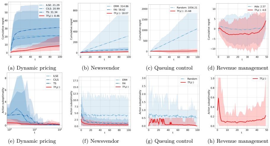
[Section 6.1.1, Figure 4 (d) and (h)] The claim that OMGPT 'consistently outperforms the structured benchmark algorithms across all tasks' is weakened by the revenue management setup, where optimal actions are approximated by the Ada algorithm and the regret is computed against an upper bound of the optimal cumulative reward. The final cumulative regret values in the legends are reported without confidence intervals or significance tests, even though the shaded areas elsewhere suggest variability. Please report credible intervals or error bars for the summary regret values and clarify how the Ada approximation affects the comparison in the revenue management task.

minor comments (6)

[Abstract and Section 1] The phrase 'pre-trained data' appears in the abstract and introduction; 'pre-training data' is the standard term and should be used consistently.
[Assumption 5.8] The first displayed condition has mismatched parentheses: the conditional expectation should be written as E[ r(X_t, Alg*(H_t)) - r(X_t, TF_hat_theta(H_t)) | H_t ] <= Delta_Exploit.
[Proposition 5.3] The proposition is stated under 'mild conditions' deferred to Appendix C, but the proof uses bounded derivatives, bounded reward/action regions, and norm bounds. These conditions should be stated explicitly in the proposition statement rather than left implicit.
[Appendix D.2] The notation Unif({0.1, 0.26, ...}) for a discrete uniform distribution is not defined; please define it or use a standard notation for uniform distributions over finite sets.
[References] The bibliography entry for Hochreiter is incomplete: 'S Hochreiter. Long short-term memory. Neural Computation MIT-Press, 1997' should include the co-author Sepp Hochreiter and the full bibliographic details.
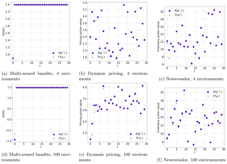
[Figure 3 caption] The caption refers to 'concentrated deviations' without specifying the aggregation: it should state how TF_hat_theta - Alg* is computed across environments and time steps, and what metric the histogram displays.

Circularity Check

2 steps flagged · score 5.0 of 10

Partial circularity: the sub-linear regret explanation assumes the exploration it claims to explain, and the revenue management benchmark is used as its own training label; the other empirical comparisons remain out-of-sample and independent.

other [Section 5.2.3, Assumption 5.8 and Example 5.10]
"we assume with some constant C, TFˆθ(Ht) = Alg∗(Ht) + ∆t, where ∆t = CT^{−1/4} w.p. 1/2, −CT^{−1/4} w.p. 1/2 for any possible history Ht and t = 1,...,T, and ∆t is independent of Ht, Alg∗(Ht), γ, and previous ∆τ for τ = 1,...,t − 1."

The paper's stated explanation of why pre-trained OMGPT avoids linear regret is that finite pre-training errors provide inherent exploration. The formal route, Theorem 5.9, requires a shrinking reward gap ∆Exploit and growth of the information matrix λt; neither is derived from the pre-training loss (11) or Algorithm 2. Example 5.10 instead assumes TF_hat_theta = Alg* + ∆t with an independent, zero-mean, symmetric ±C T^{-1/4} perturbation — exactly the exploration structure needed to make λt grow and ∆Exploit = O(T^{-1/2}). The O(d√T) regret is therefore a consequence of assuming the exploration phenomenon, not of the pre-training procedure.
fitted input called prediction [Section 6.1.1 and Figure 4 caption (revenue management)]
"For revenue management, since the exact optimal actions are computed at a high computation cost, we use the actions from the Adaptive Allocation Algorithm (Ada) from Chen et al. [2024], which can achieve constant regret, to approximate optimal actions in both the pre-training and testing (and thus not show the suboptimality of the Ada algorithm in (h)), and use their upper bound of the optimal cumulative reward to compute (an upper bound) of the regret used in (d)."

In this panel, the 'optimal actions' used as supervised labels are generated by the same Ada algorithm that is the comparison benchmark. Section 6.1.1 then concludes that TF_hat_theta 'uncovers a new and more effective approach' and 'consistently outperforms the structured benchmark algorithms across all tasks.' For revenue management, the model is trained to imitate the benchmark's decisions, so the outperformance claim is not an independent out-of-sample discovery; the benchmark's rule is baked into the training target. This is disclosed in the caption, but it makes that specific panel's evidence partly circular, although it does not affect the other three tasks where optimal actions are computed analytically.

full rationale

The main numerical claim on dynamic pricing, newsvendor, and queueing control compares TF_hat_theta against standard external algorithms on out-of-sample environments, so that core empirical comparison is self-contained and not circular. Proposition 5.1 is essentially definitional, since Alg* is constructed as the pointwise minimizer of the same expected loss, but it is not used to force the numerical results. The regret analysis is explicitly conditional: Theorem 5.9 holds under Assumption 5.8, and Example 5.10 is labeled a stylized model. The circular element is that the paper's narrative explanation — finite pre-training errors provide inherent exploration — is not derived from pre-training; the example simply assumes the exploration-friendly perturbation. In addition, the revenue management panel uses Ada actions as both the training labels and the benchmark, so that particular 'outperforms all benchmarks' claim is partly self-referential. These are partial circularities confined to the theoretical explanation and one experiment; the overall framework still has substantial independent empirical content.

Assumptions & free parameters 3 free parameters · 6 assumptions · 0 invented entities

The central claim rests on a prior over environments, computable optimal-action labels, a rich transformer class, and regularity assumptions on the observation model. The regret theorem additionally assumes the trained model is already close to Bayes-optimal (Delta_Exploit) and that its errors provide KL information (Delta_Explore), neither of which is proved. This is the main gap between the empirical demonstration and the claimed guarantees.

free parameters (3)

Delta_Exploit (Assumption 5.8) = not estimated
Assumed constant upper bound on the reward gap between TF_hat_theta and Alg* at every history. The regret bound in Theorem 5.9 is linear in this constant, and the paper derives no value for it from pretraining.
Delta_Explore (Assumption 5.7 and 5.8) = not estimated
Assumed lower bound on KL divergence per unit parameter distance under TF_hat_theta's action distribution. No result establishes this for the trained transformer; it is the exploration intensity that makes the bound sublinear.
Perturbation amplitude in Example 5.10 = C T^{-1/4} with probability 1/2 for each sign
Example 5.10 postulates TF_hat_theta = Alg* plus this symmetric noise to obtain O(sqrt(T)) regret. This deviation profile is chosen by hand, not derived from the pretraining objective.

assumptions (6)

domain assumption Decision maker has a known prior distribution P_gamma over environments and can sample gamma_i from it.
Used throughout Section 4.3.1 to generate pretraining environments. If the prior is misspecified, pretraining data no longer represents test environments, and the paper's own out-of-domain experiments show performance degradation at large shifts.
domain assumption Optimal action a*_t can be computed for each sampled environment gamma_i.
Section 4.3.1 labels pretraining samples with a*_t computed from the known simulated environment. This requires a simulator or known parametric family, which may not be available in real applications.
ad hoc to paper The transformer function class F is rich enough to contain Alg*, and infinite pretraining data would make the empirical minimizer equal to Alg*.
Section 5.1 states this conditional assumption explicitly. No finite-sample or approximation-error result is provided, so the connection between TF_hat_theta and Alg* is not guaranteed.
domain assumption Assumption 5.7: observation log-likelihood has a KL lower bound, sub-Gaussian log-ratio, concavity in gamma, and bounded Hessian.
These conditions drive posterior concentration in Theorem 5.9 and are satisfied for Gaussian linear demand, but not for all OR tasks studied numerically, such as censored newsvendor or queueing control.
ad hoc to paper Assumption 5.8: TF_hat_theta is within Delta_Exploit reward of Alg*, and Alg*'s reward gap is controlled by posterior variance.
This is the main assumption that turns the regret bound into a meaningful statement. It is asserted about the trained model and is not derived from the pretraining loss or data generation.
domain assumption Assumption 5.6: environment space is bounded, rewards are bounded, and P_gamma is uniform over Gamma.
Standard regularity for regret analysis; the paper notes the uniformity can be relaxed at the cost of a likelihood-ratio multiplier.

how reviews work

0 comments

Cite this review

Pith. "Pith review of OMGPT: A Sequence Modeling Framework for Data-driven Operational Decision Making." pith.science (2026). https://pith.science/paper/H46YXYHI

@misc{pith2026250513580,
  author       = {Pith},
  title        = {Pith review of: OMGPT: A Sequence Modeling Framework for Data-driven Operational Decision Making},
  year         = {2026},
  howpublished = {\url{https://pith.science/paper/H46YXYHI}},
  note         = {Machine review of arXiv:2505.13580}
}

read the original abstract

We build a Generative Pre-trained Transformer (GPT) model from scratch to solve sequential decision making tasks arising in contexts of operations research and management science which we call OMGPT. We first propose a general sequence modeling framework to cover several operational decision making tasks as special cases, such as dynamic pricing, inventory management, resource allocation, and queueing control. Under the framework, all these tasks can be viewed as a sequential prediction problem where the goal is to predict the optimal future action given all the historical information. Then we train a transformer-based neural network model (OMGPT) as a natural and powerful architecture for sequential modeling. This marks a paradigm shift compared to the existing methods for these OR/OM tasks in that (i) the OMGPT model can take advantage of the huge amount of pre-trained data; (ii) when tackling these problems, OMGPT does not assume any analytical model structure and enables a direct and rich mapping from the history to the future actions. Either of these two aspects, to the best of our knowledge, is not achieved by any existing method. We establish a Bayesian perspective to theoretically understand the working mechanism of the OMGPT on these tasks, which relates its performance with the pre-training task diversity and the divergence between the testing task and pre-training tasks. Numerically, we observe a surprising performance of the proposed model across all the above tasks.

Figures

Figures reproduced from arXiv: 2505.13580 by the authors.

**Figure 2.** The testing/application phase of the pre-trained OMGPT. we iteratively input the history [PITH_FULL_IMAGE:figures/full_fig_p010_2.png] view at source ↗

**Figure 3.** TFθˆ nearly matches the optimal decision function Alg∗ in dynamic pricing tasks with concentrated deviations. Figure (a) shows one decision trial for Alg∗ and TFθˆ ,where the optimal actions change over time because Xt’s are different for different time t. Figure (b) shows the histogram of TFθˆ − Alg∗ over different environments. The experiment setup and more results are deferred to Appendix D.1.1. In addition, the … view at source ↗

Figures from the paper (22 more)

**Figure 4.** Figure 4: The average out-of-sample regret (first row) and action suboptimality, i.e., |a ∗ t −Alg(Ht)|, (second row) of TFθˆ against benchmark algorithms (see details in Appendix D.3). The numbers in the legend bar are the final cumulative regret. The last two tasks can have ne…

**Figure 5.** Figure 5: The advantage of OMGPT compared to the best benchmark algorithm in dynamic pricing, [PITH_FULL_IMAGE:figures/full_fig_p023_5.png]

**Figure 6.** Figure 6: Performance under horizon generalization in newsvendor problems with uncensored and cen [PITH_FULL_IMAGE:figures/full_fig_p024_6.png]

**Figure 7.** Figure 7: Performance under different testing noise variances, which may deviate from the pre-training [PITH_FULL_IMAGE:figures/full_fig_p025_7.png]

**Figure 8.** Figure 8: Performance under the different levels of out-of-domain shifts [PITH_FULL_IMAGE:figures/full_fig_p026_8.png]

**Figure 9.** Figure 9: Performance under the different levels of in-domain shifts [PITH_FULL_IMAGE:figures/full_fig_p026_9.png]

**Figure 10.** Figure 10: Performance in stationary environments ((a), (c)) and non-stationary environments ((b), (d)), [PITH_FULL_IMAGE:figures/full_fig_p028_10.png]

**Figure 11.** Figure 11: Performance in environments with linear demand ((a), (c)) and environments with square [PITH_FULL_IMAGE:figures/full_fig_p029_11.png]

**Figure 12.** Figure 12: Out-of-sample demand prediction error comparison between OMGPT ( [PITH_FULL_IMAGE:figures/full_fig_p030_12.png]

**Figure 13.** Figure 13: Visualization of output embedding vectors from different layers. The vectors corresponding [PITH_FULL_IMAGE:figures/full_fig_p031_13.png]

**Figure 14.** Figure 14: Normalized prediction errors of demand type, demand parameters, and optimal actions across [PITH_FULL_IMAGE:figures/full_fig_p032_14.png]

**Figure 15.** Figure 15: (a) Histogram of optimal action changes due to the manipulation of the context [PITH_FULL_IMAGE:figures/full_fig_p033_15.png]

**Figure 16.** Figure 16: The architecture of OMGPT, where all actions [PITH_FULL_IMAGE:figures/full_fig_p038_16.png]

**Figure 17.** Figure 17: Performances of TFθˆ and oracle posterior algorithms. The numbers in the legend bar are the final regret at t = 100 and the shaded areas indicate the 90% (empirical) confidence intervals. short-term regret than oracle posterior algorithms. It can be more greedy than p…

**Figure 18.** Figure 18: (a) Training dynamics. Orange: M0 = M = 130. Blue: M0 = 50 and M = 130. It shows the effectiveness of injecting/mixing the transformer-generated sequence into the training procedure. (b) A visualization of the Ht with aτ ’s in Ht generated from various TFθm. For each …

**Figure 19.** Figure 19: (a) The effect of ˜f (decision function for generating the pre-training data), where we mix the UCB algorithm [Lattimore and Szepesvári, 2020] and decision function (20) with different ratios to create the pre-training data. (b) The effect of κ (ratio of samples gener…

**Figure 20.** Figure 20: Examples to compare the actions from the transformer [PITH_FULL_IMAGE:figures/full_fig_p061_20.png]

**Figure 21.** Figure 21: TFθˆ(Ht) − Alg∗ (Ht) across different tasks with various numbers of possible environments. More possible environments lead to a harder decision making problem. 61 [PITH_FULL_IMAGE:figures/full_fig_p061_21.png]

**Figure 22.** Figure 22: The average out-of-sample regret on tasks with simpler environments, where each task only [PITH_FULL_IMAGE:figures/full_fig_p062_22.png]

**Figure 23.** Figure 23: The average out-of-sample regret on harder tasks: with 100 environments in (a) multi-armed [PITH_FULL_IMAGE:figures/full_fig_p062_23.png]

**Figure 24.** Figure 24: Comparison of the average out-of-sample regret between using the Transformer and LSTM [PITH_FULL_IMAGE:figures/full_fig_p063_24.png]

**Figure 25.** Figure 25: Complete results corresponding to Figure [PITH_FULL_IMAGE:figures/full_fig_p070_25.png]

Discussion (0). Continue with ORCID to comment.

Forward citations

Cited by 1 Pith paper

Reviewed papers in the Pith corpus that reference this work. Sorted by Pith novelty score. Full citation record

LLM-SAA: LLM-persona Generated Distributions for Decision-making
cs.LG 2026-02 conditional novelty 7.0 of 10

LLM-generated distributions used in sample-average optimization give competitive decisions in low-data regimes, and decision-agnostic distances like Wasserstein misjudge their quality.

Reference graph

Works this paper leans on

38 extracted references · 21 canonical work pages · cited by 1 Pith paper

[1]

+λt−1) λt−1 min{√ϵt, 1} !d   where the first line is from the definition of the packing number, the second line comes from the relation- ship between covering and packing numbers (Lemma 4.2.8 in [Vershynin, 2018]), the third line is from the definition ofϵ′, the fourth line is byϵt≤ϵ, and the last line is from Example 27.1 in Shalev-Shwartz and Ben-David

work page 2018
[2]

Understanding intermediate layers using linear classifier probes

Guillaume Alain. Understanding intermediate layers using linear classifier probes. arXiv preprint arXiv:1610.01644,

arXiv
[3]

Algorithm 3Adaptive Allocation Algorithm[Chen et al., 2024] 1: Input: T,X ={(˜rk, ˜Ak)}K k=1 2: Initialize B1 =T· 1, b1 = B1/T 3: Set y1 = 1 4: for t = 2,...,T do 5: Compute Bt = Bt−1− ˜At−1yt−1 6: Compute bt = Bt/(T−t +

work page 2024
[4]

following the sampling rules previously described

i.i.d. following the sampling rules previously described. We then set the environment distributionPγ as a uniform distribution over the pool of sampled environments (e.g., {γ1,...,γ 4}). We should notice this pool of environments does not restrict the context generation (if any): in both the pre-training and testing, contexts are generated following the r...

work page 2020
[5]

Rvs: What is essential for offline rl via supervised learning?arXiv preprint arXiv:2112.10751,

Scott Emmons, Benjamin Eysenbach, Ilya Kostrikov, and Sergey Levine. Rvs: What is essential for offline rl via supervised learning?arXiv preprint arXiv:2112.10751,

arXiv
[9]

Scaling laws for neural language models.arXiv preprint arXiv:2001.08361,

Jared Kaplan, Sam McCandlish, Tom Henighan, Tom B Brown, Benjamin Chess, Rewon Child, Scott Gray, Alec Radford, Jeffrey Wu, and Dario Amodei. Scaling laws for neural language models.arXiv preprint arXiv:2001.08361,

arXiv 2001
[11]

Transformers as decision makers: Provable in-context reinforcement learning via supervised pretraining.arXiv preprint arXiv:2310.08566,

36 Licong Lin, Yu Bai, and Song Mei. Transformers as decision makers: Provable in-context reinforcement learning via supervised pretraining.arXiv preprint arXiv:2310.08566,

arXiv
[16]

An explanation of in-context learning as implicit bayesian inference.arXiv preprint arXiv:2111.02080,

Sang Michael Xie, Aditi Raghunathan, Percy Liang, and Tengyu Ma. An explanation of in-context learning as implicit bayesian inference.arXiv preprint arXiv:2111.02080,

arXiv

Show all 38 references

[17]

Closing the gap: A learning algorithm for lost-sales inventory systems with lead times.Management Science, 66(5):1962–1980,

Huanan Zhang, Xiuli Chao, and Cong Shi. Closing the gap: A learning algorithm for lost-sales inventory systems with lead times.Management Science, 66(5):1962–1980,

1962
[18]

What and how does in-context learning learn? bayesian model averaging, parameterization, and generalization

Yufeng Zhang, Fengzhuo Zhang, Zhuoran Yang, and Zhaoran Wang. What and how does in-context learning learn? bayesian model averaging, parameterization, and generalization. arXiv preprint arXiv:2305.19420,

arXiv
[19]

A survey of large language models.arXiv preprint arXiv:2303.18223,

Wayne Xin Zhao, Kun Zhou, Junyi Li, Tianyi Tang, Xiaolei Wang, Yupeng Hou, Yingqian Min, Be- ichen Zhang, Junjie Zhang, Zican Dong, et al. A survey of large language models.arXiv preprint arXiv:2303.18223,

arXiv
[20]

label type

Input Sequence Structure.Since we have three types of elements (contexts, actions, and observa- tions), and the actions are the “label type” we want to predict sequentially, we first combine the contexts and the observations into “features”, similar to a supervised learning ta...

2018
[21]

informing

propose constructing input sequences for predictinga∗ t using a set of tuples (Xτ,aτ,Oτ,Xτ+1), which are sampled from a trajectory and are not contiguous or in chronological order. Intuitively, the goal is for the pre-trained transformer to implicitly learn the transitions and...

2014
[22]

39 • GPTmodelarchitecture: Duetothedifferentdatagenerationmethodsandthespecialstructure of the underlying problems, we employ a different GPT architecture

focuses primarily on problems with discrete action spaces, whereas we conduct experiments and provide analyses for both discrete and continuous action spaces. 39 • GPTmodelarchitecture: Duetothedifferentdatagenerationmethodsandthespecialstructure of the underlying problems, we...

2022
[24]

However, we do not encounter this instability in our numerical experiment, and we make an argument as the following claim

shows that the matter can be solved with strong conditions such as smoothness and strong convexity on the objective function. However, we do not encounter this instability in our numerical experiment, and we make an argument as the following claim. That is, when the underlying...

2020
[25]

TX t=1 l(f(Ht),a∗ t ) # = E

B.3 More Experiments on Pre-training In this section, we present ablation studies to explore the impact of two key factors: the decision function ˜f usedforgeneratingpre-trainingdata, andthemixratio κappliedinAlgorithm2. Figure19summarizes the results, where we pre-train and t...

2020
[26]

exploration intensity

C.4 Proof and Discussions of Theorem 5.9 We first introduce a few key lemmas for proving Theorem 5.9. We denotePt(·) = Pγ(·|Ht), i.e., the posterior distribution of the (testing) environment at timet, which generatesHt through (12), condi- tional on the historyHt. And let Et[·...

2014
[27]

Thus, by the union bound, for allt≥ max{512(¯a +C)2C4 log2T √ T, 4C2 log(dT

and the analysis in Example 1 of Keskin and Zeevi [2014], for eacht, there exist constantsC1,C 2 > 0, related to the boundedness of the parameters, such that with probability at least1−d exp −C1 Pt τ=2(aτ− ¯aτ−1)2 , λt≥C2 tX τ=2 (aτ− ¯aτ−1)2. Thus, by the union bound, for allt...

2014
[28]

C.4.5 Proofs of Lemmas Proof for Lemma C.1 Proof

a2 + TX t=2 4Cr (t− 1)a2 =O(logT ) which completes the proof. C.4.5 Proofs of Lemmas Proof for Lemma C.1 Proof. By the Bernstein-type concentration bound for a martingale difference sequence (Theorem 2.19 in [Wainwright, 2019]), under Assumption 5.7, we have for anyγ′∈ Γ,t> 0 ...

2019
[30]

For Figure 20, each subfigure is based on a sampled environment with a sampled sequence of contexts{Xt}30 t=1 from the corresponding task

Setup. For Figure 20, each subfigure is based on a sampled environment with a sampled sequence of contexts{Xt}30 t=1 from the corresponding task. The data generation process follows the description detailed in Appendix D.2. Both the pre-training and testing samples are drawn f...

1997
[31]

The optimal arm isa∗ = arg maxara

for each actiona. The optimal arm isa∗ = arg maxara. Linear bandits There is no context, i.e.,Xt = null for allt. The action at∈A⊂ Rd is selected from some pre-specified domainA. The random rewardR(Xt,at) = w⊤at +ϵt where ϵt is some zero- mean noise random variable andw∈ Rd is...

2024
[32]

Then right before the end of the time period, one customer will arrive with an unknown arrival rateλ

At the beginning of each time periodt, the decision maker can first observe the length of queue, and then decide the service rateat∈{ 0, 0.2,..., 1} to process the customers in the queue. Then right before the end of the time period, one customer will arrive with an unknown ar...

2006
[34]

D.3.2 Linear bandits • LinUCB [Chu et al., 2011]: GivenHt, we defineΣt =Pt−1 τ=1aτa⊤ τ +σ2Id, whereσ2 is the variance of the reward noise

The posterior distribution can be computed by P(γi|Ht) = exp(− 1 σ2 Pt−1 τ=1(Oτ−ri aτ )2) P|Γ| i′=1 exp(− 1 σ2 Pt−1 τ=1(Oτ−ri′ aτ )2) , where ri a is the expected reward ofa in environmentγi and σ2 is the variance of the noise (which equals to 0.2 in our experiments). D.3.2 Li...

2011
[35]

feature vector

The posterior distribution can be computed by P(γi|Ht) = exp(− 1 σ2 Pt−1 τ=1(Oτ−w⊤ i aτ)2) P|Γ| i′=1 exp(− 1 σ2 Pt−1 τ=1(Oτ−w⊤ i′aτ)2) , where wi is the reward function parameter in environmentγi and σ2 is the variance of the noise (which equals to0.2 in our experiments). D.3....

2016
[36]

To compute the posterior distribution, we follow the notations in ILSE and denotew = (α,β ) as the stacked vector of parameters, then the posterior distribution is P(γi|Ht) = exp(− 1 σ2 Pt−1 τ=1(Oτ−w⊤ i zτ)2) P|Γ| i′=1 exp(− 1 σ2 Pt−1 τ=1(Oτ−w⊤ i′zτ)2) , where wi is the demand...

2019
[37]

Then the posterior distribution of the underlying environment is P(γi|Ht) = 1 ¯Eγi,t· ¯ϵ1−t γi P|Γ| i′=1 1 ¯Eγi′,t· ¯ϵ1−tγi′

To compute the posterior distribution, we denote ¯ϵγ and βγ as the noise upper bound and demand function parameter ofγ at τ≤t− 1, and define 68 the eventEγ,τ = n 0≤Oτ−β⊤ γ ˜Xτ≤ ¯ϵ o to indicate the feasibility of environmentγ from ( ˜Xτ,Oτ), and denote ¯Eγ,t =Tτ−1 τ=1Eγ,τ to i...

2024
[130]

E(Ht,a∗ t )∼κPγ, ˜f+(1−κ)Pγ,TFθ

It shows the effectiveness of injecting/mixing the transformer-generated sequence into the training procedure. (b) A visualization of theHt with aτ’s inHt generated from variousTFθm. For each TFθm, we generate 30 sequences. The decision functionAlg∗ is defined in the next sect...

2020
[2001]

Deep neural newsvendor.arXiv preprint arXiv:2309.13830,

Jinhui Han, Ming Hu, and Guohao Shen. Deep neural newsvendor.arXiv preprint arXiv:2309.13830,

arXiv
[2012]

Gaussian error linear units (gelus).arXiv preprint arXiv:1606.08415,

Dan Hendrycks and Kevin Gimpel. Gaussian error linear units (gelus).arXiv preprint arXiv:1606.08415,

arXiv
[2014]

In-context reinforcement learning with algorithm distillation.arXiv preprint arXiv:2210.14215,

Michael Laskin, Luyu Wang, Junhyuk Oh, Emilio Parisotto, Stephen Spencer, Richie Steigerwald, DJ Strouse, Steven Hansen, Angelos Filos, Ethan Brooks, et al. In-context reinforcement learning with algorithm distillation.arXiv preprint arXiv:2210.14215,

arXiv
[2015]

An information-theoretic analysis of in-context learning

Hong Jun Jeon, Jason D Lee, Qi Lei, and Benjamin Van Roy. An information-theoretic analysis of in-context learning. arXiv preprint arXiv:2401.15530,

arXiv
[2016]

Representing random utility choice models with neural networks.arXiv preprint arXiv:2207.12877,

Ali Aouad and Antoine Désir. Representing random utility choice models with neural networks.arXiv preprint arXiv:2207.12877,

arXiv
[2019]

On dynamic pricing with covariates.arXiv preprint arXiv:2112.13254,

Hanzhao Wang, Kalyan Talluri, and Xiaocheng Li. On dynamic pricing with covariates.arXiv preprint arXiv:2112.13254,

arXiv
[2020]

Reinforcement learning for intensity control: An application to choice-based network revenue management.arXiv preprint arXiv:2406.05358,

Huiling Meng, Ningyuan Chen, and Xuefeng Gao. Reinforcement learning for intensity control: An application to choice-based network revenue management.arXiv preprint arXiv:2406.05358,

arXiv
[2021]

A neural network based choice model for assortment optimization.arXiv preprint arXiv:2308.05617,

Hanzhao Wang, Zhongze Cai, Xiaocheng Li, and Kalyan Talluri. A neural network based choice model for assortment optimization.arXiv preprint arXiv:2308.05617,

arXiv
[2022]

Is conditional generative modeling all you need for decision-making?arXiv preprint arXiv:2211.15657,

Anurag Ajay, Yilun Du, Abhi Gupta, Joshua Tenenbaum, Tommi Jaakkola, and Pulkit Agrawal. Is conditional generative modeling all you need for decision-making?arXiv preprint arXiv:2211.15657,

arXiv
[2023]

Dynamic pricing with demand covariates

Sheng Qiang and Mohsen Bayati. Dynamic pricing with demand covariates. arXiv preprint arXiv:1604.07463,

arXiv
[2024]

A survey on in-context learning.arXiv preprint arXiv:2301.00234,

Qingxiu Dong, Lei Li, Damai Dai, Ce Zheng, Jingyuan Ma, Rui Li, Heming Xia, Jingjing Xu, Zhiyong Wu, Tianyu Liu, et al. A survey on in-context learning.arXiv preprint arXiv:2301.00234,

arXiv

Pith tools

Reviewed August 15, 2026 · model on record in the stance chip above.

[1] [1]

+λt−1) λt−1 min{√ϵt, 1} !d   where the first line is from the definition of the packing number, the second line comes from the relation- ship between covering and packing numbers (Lemma 4.2.8 in [Vershynin, 2018]), the third line is from the definition ofϵ′, the fourth line is byϵt≤ϵ, and the last line is from Example 27.1 in Shalev-Shwartz and Ben-David

work page 2018

[2] [2]

Understanding intermediate layers using linear classifier probes

Guillaume Alain. Understanding intermediate layers using linear classifier probes. arXiv preprint arXiv:1610.01644,

arXiv

[3] [3]

Algorithm 3Adaptive Allocation Algorithm[Chen et al., 2024] 1: Input: T,X ={(˜rk, ˜Ak)}K k=1 2: Initialize B1 =T· 1, b1 = B1/T 3: Set y1 = 1 4: for t = 2,...,T do 5: Compute Bt = Bt−1− ˜At−1yt−1 6: Compute bt = Bt/(T−t +

work page 2024

[4] [4]

following the sampling rules previously described

i.i.d. following the sampling rules previously described. We then set the environment distributionPγ as a uniform distribution over the pool of sampled environments (e.g., {γ1,...,γ 4}). We should notice this pool of environments does not restrict the context generation (if any): in both the pre-training and testing, contexts are generated following the r...

work page 2020

[5] [5]

Rvs: What is essential for offline rl via supervised learning?arXiv preprint arXiv:2112.10751,

Scott Emmons, Benjamin Eysenbach, Ilya Kostrikov, and Sergey Levine. Rvs: What is essential for offline rl via supervised learning?arXiv preprint arXiv:2112.10751,

arXiv

[6] [9]

Scaling laws for neural language models.arXiv preprint arXiv:2001.08361,

Jared Kaplan, Sam McCandlish, Tom Henighan, Tom B Brown, Benjamin Chess, Rewon Child, Scott Gray, Alec Radford, Jeffrey Wu, and Dario Amodei. Scaling laws for neural language models.arXiv preprint arXiv:2001.08361,

arXiv 2001

[7] [11]

Transformers as decision makers: Provable in-context reinforcement learning via supervised pretraining.arXiv preprint arXiv:2310.08566,

36 Licong Lin, Yu Bai, and Song Mei. Transformers as decision makers: Provable in-context reinforcement learning via supervised pretraining.arXiv preprint arXiv:2310.08566,

arXiv

[8] [16]

An explanation of in-context learning as implicit bayesian inference.arXiv preprint arXiv:2111.02080,

Sang Michael Xie, Aditi Raghunathan, Percy Liang, and Tengyu Ma. An explanation of in-context learning as implicit bayesian inference.arXiv preprint arXiv:2111.02080,

arXiv