The Landscape of Composite Higgs Models
Pith reviewed 2026-06-26 23:34 UTC · model grok-4.3
The pith
A Bayesian tuning measure applied to Composite Higgs models finds limited naturalness improvements from common extensions.
A machine-rendered reading of the paper's core claim, the machinery that carries it, and where it could break.
Core claim
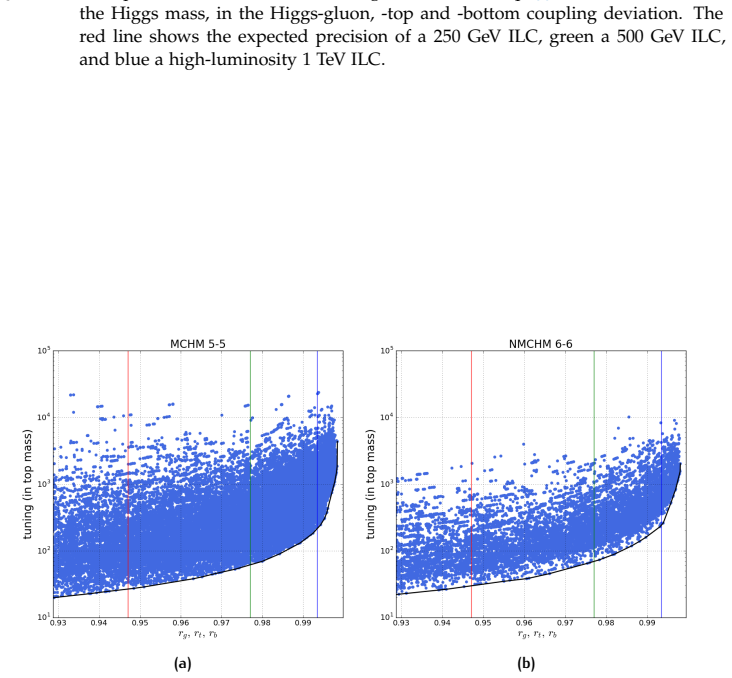
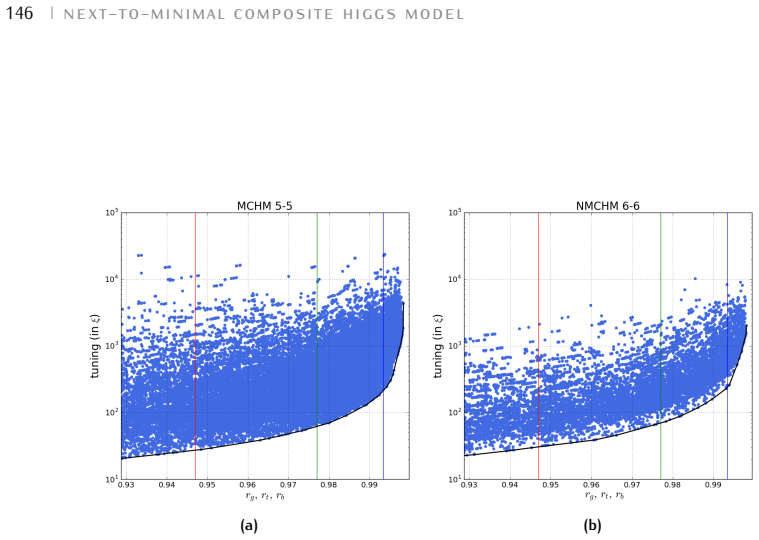
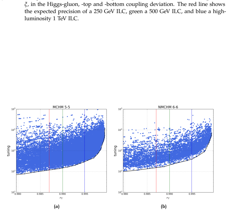
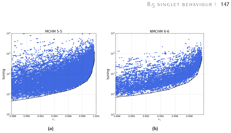
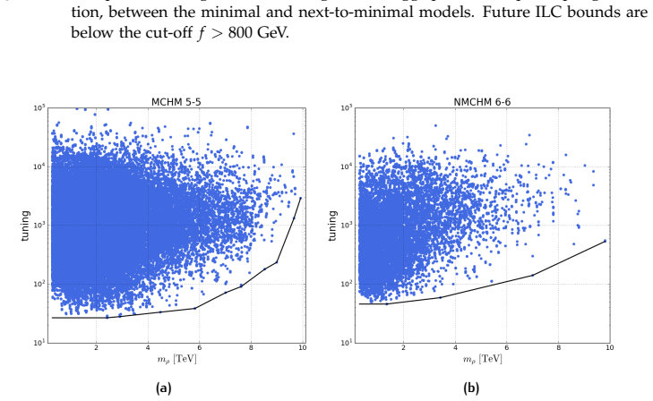
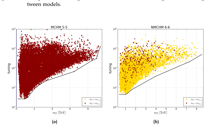
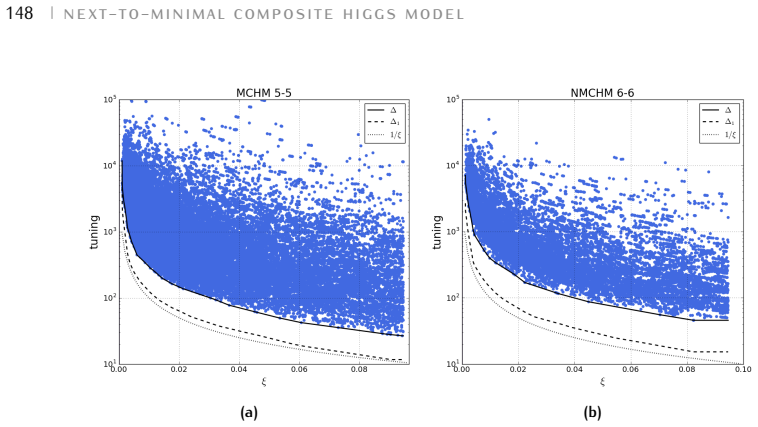
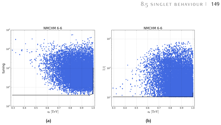
Through global fits and the application of the new tuning measure, the work concludes that extensions to the minimal 4D composite Higgs model, such as embedding a composite tau or adding a dark matter candidate, provide no substantial benefit to naturalness in the composite Higgs sector.
What carries the argument
The N-site four-dimensional composite Higgs model, an effective theory where the Higgs emerges as a pseudo-Goldstone boson from a strong dynamics sector at higher scales, combined with the proposed Bayesian tuning measure that quantifies the improbability of the observed Higgs mass parameter.
If this is right
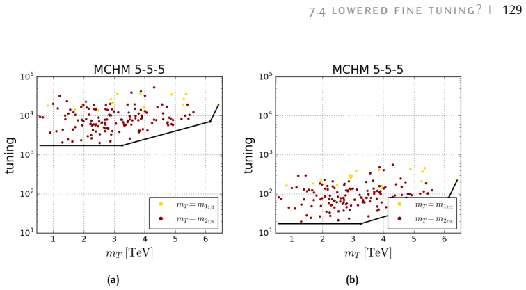
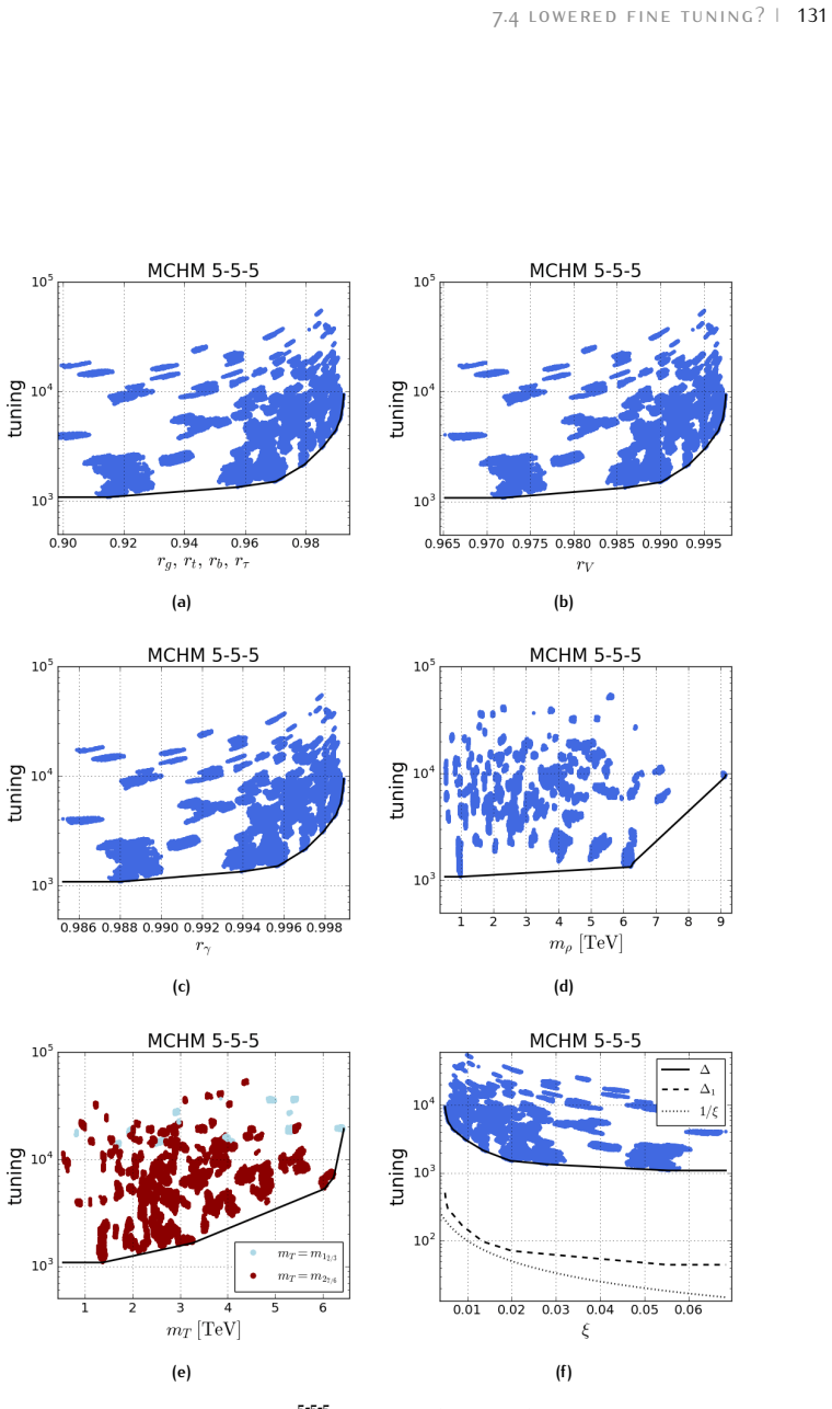
- Collider searches impose strong exclusion limits on the minimal model's parameters.
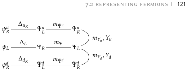
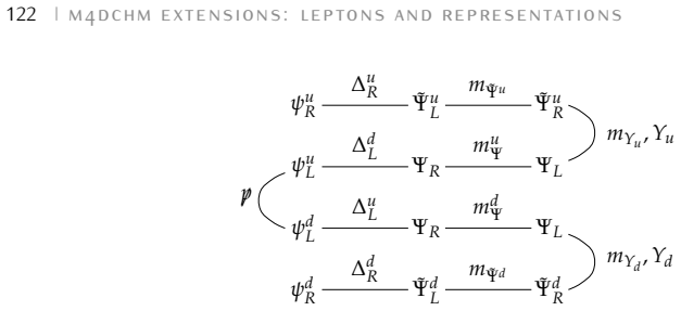
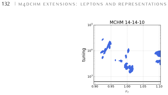
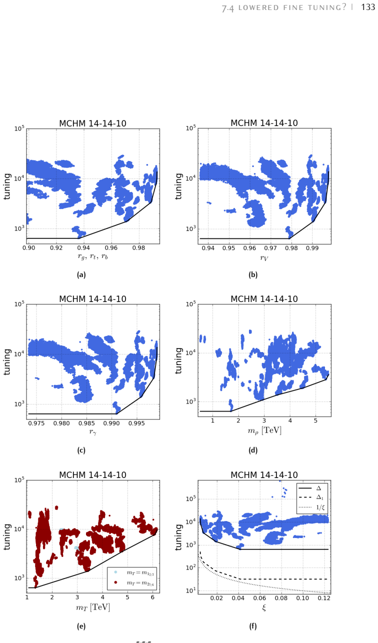
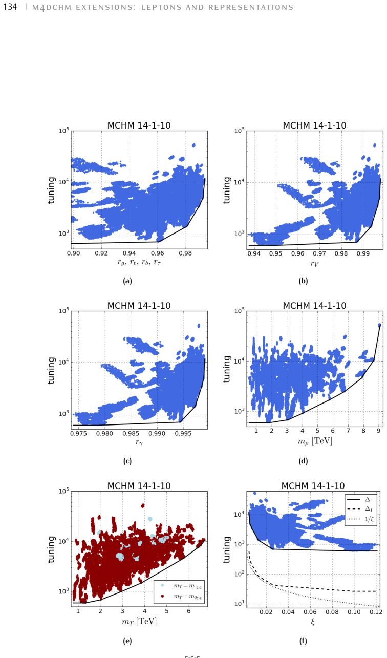
- Embedding composite leptons in different representations yields no significant reduction in tuning.
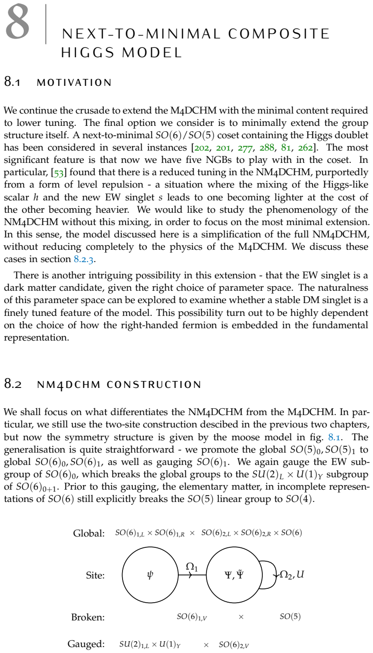
- The next-to-minimal model with a dark matter candidate shows comparable or worse naturalness metrics.
- The Bayesian tuning measure allows quantitative comparison of naturalness across different composite Higgs setups.
Where Pith is reading between the lines
- The results imply that achieving better naturalness may require going beyond these simple extensions to more intricate model structures.
- The measure could be tested for consistency by applying it to other beyond-Standard-Model scenarios with known naturalness properties.
- Collider experiments might prioritize searches motivated by other considerations if naturalness gains remain minimal.
Load-bearing premise
The new tuning measure correctly captures the concept of naturalness in a way that matches physical intuition and that the four-dimensional models sufficiently describe the relevant physics at collider energies.
What would settle it
A future collider observation of a light composite resonance whose parameters require extreme tuning according to the measure but appear in data would challenge the exclusion bounds and naturalness conclusions.
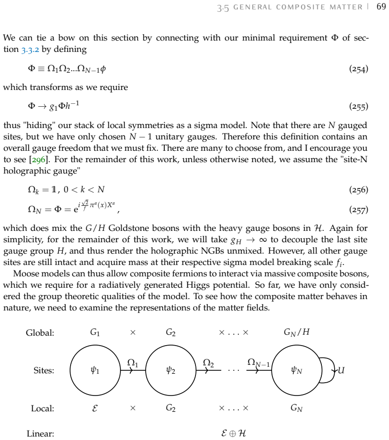
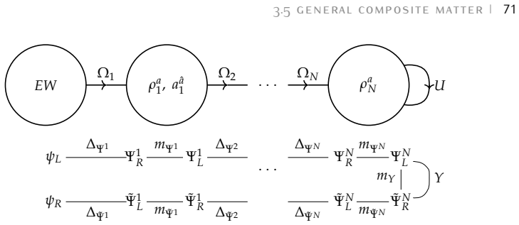
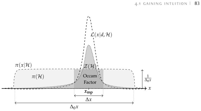
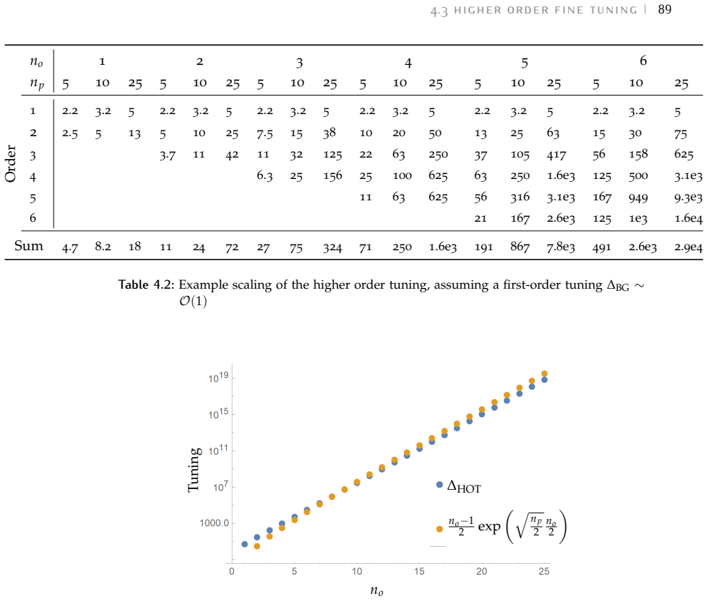
Figures

read the original abstract
While the Standard Model (SM) of particle physics contains the most precise set of predictions ever devised by humanity, that precision comes at a cost. The strange nature of the Higgs particle requires its parameters to be tuned so precisely that if the SM is indeed the true description of reality, one is forced to wonder how such a miracle as galactic structure and life could occur. Instead, we search in this work for a natural explanation. The concept of naturalness is comprehensively explored, and a new tuning measure proposed, with an aim to place it on well-defined Bayesian footing. We then turn this measure on to the analysis of a class of intriguing new physics - Composite Higgs models. These effective models are the result of a plethora of underlying theories, and they allow the production of a naturally light Higgs particle, appearing as the SM Higgs at low energy. We establish the background required to appreciate the N-site 4D Composite Higgs model, and subsequently focus on the simplest incarnations of this class. A global fit is performed on the Minimal 4D Composite Higgs model (M4DCHM), with strong exclusion bounds placed on collider search channels. We analyse any improvement in tuning that could be gained from several extensions to this model. The Leptonic M4DCHM is explored, with a composite tau lepton embedded in various representations. The possibility of a dark matter candidate existing in the Next-to-Minimal 4DCHM is considered. Ultimately, we are able to define what, if any, benefit to naturalness can come to the Composite Higgs sector by introducing these extensions.
Editorial analysis
A structured set of objections, weighed in public.
Referee Report
Summary. The manuscript proposes a new tuning measure intended to place naturalness on Bayesian footing, applies it to the Minimal 4D Composite Higgs Model (M4DCHM) through a global fit that yields strong exclusion bounds on collider channels, and examines whether leptonic extensions or the Next-to-Minimal 4DCHM improve the tuning relative to the baseline, ultimately assessing any naturalness benefit from these extensions.
Significance. If the tuning measure is rigorously derived from well-motivated priors and the global fits are reproducible, the work would supply a quantitative framework for comparing naturalness across composite Higgs scenarios and their extensions, clarifying whether leptonic or dark-matter extensions yield measurable improvement.
major comments (2)
- [Tuning measure section] The section introducing the tuning measure asserts that it places naturalness on well-defined Bayesian footing, yet provides no explicit derivation of the prior on the Higgs-mass parameter or composite scale, no marginal-likelihood expression, and no demonstration that the measure alters posterior odds rather than reproducing a conventional fine-tuning metric.
- [Global fit section] The global-fit section reports strong exclusion bounds on collider search channels for the M4DCHM but supplies no description of the data sets employed, the treatment of experimental and theoretical errors, or the statistical procedure used to obtain the posterior, rendering the bounds impossible to assess or reproduce.
Simulated Author's Rebuttal
We thank the referee for the careful and constructive review. The comments identify key areas where additional detail is needed to support the claims regarding the Bayesian tuning measure and the reproducibility of the global fit. We address each point below and will revise the manuscript to incorporate the requested clarifications.
read point-by-point responses
-
Referee: [Tuning measure section] The section introducing the tuning measure asserts that it places naturalness on well-defined Bayesian footing, yet provides no explicit derivation of the prior on the Higgs-mass parameter or composite scale, no marginal-likelihood expression, and no demonstration that the measure alters posterior odds rather than reproducing a conventional fine-tuning metric.
Authors: We agree that the derivation of the priors on the Higgs-mass parameter and composite scale, along with the marginal-likelihood expression and explicit comparison to posterior odds, requires more detail to fully substantiate the Bayesian foundation. In the revised manuscript we will add a dedicated subsection that derives the prior choices from first principles, presents the marginal likelihood explicitly, and demonstrates how the measure modifies posterior odds relative to conventional fine-tuning metrics, including the relevant equations and prior justification. revision: yes
-
Referee: [Global fit section] The global-fit section reports strong exclusion bounds on collider search channels for the M4DCHM but supplies no description of the data sets employed, the treatment of experimental and theoretical errors, or the statistical procedure used to obtain the posterior, rendering the bounds impossible to assess or reproduce.
Authors: We acknowledge that the absence of explicit information on the datasets, uncertainty treatment, and statistical procedure limits reproducibility. The revised version will include a new subsection detailing the specific collider datasets employed, the incorporation of experimental and theoretical uncertainties into the likelihood function, and the full Bayesian inference procedure used to obtain the posterior, including sampling methods, to enable assessment and reproduction of the reported bounds. revision: yes
Circularity Check
No significant circularity; derivation self-contained against external benchmarks
full rationale
The abstract introduces a new tuning measure aimed at Bayesian footing and applies it to global fits of the M4DCHM and extensions, but the provided text contains no equations, self-citations, or derivations that reduce the measure or naturalness benefit to a fit or prior result by construction. No load-bearing self-citation chain or self-definitional step is exhibited. The central claim remains independent of its own inputs per the available content, consistent with the most common honest finding of no circularity.
Axiom & Free-Parameter Ledger
Reference graph
Works this paper leans on
-
[1]
(606) for a volume spanned by three vectors
Now,du 1 1 is just a scalar, and it can be factored out of the square root Vol(f(dP)) = vuuuut (J1)o 1(J1)o 1 (J1)p 1 (J2)p 2 (J1)q 1(J3)q 3 (J2)o 2(J1)o 1 (J2)p 2 (J2)p 2 (J2)q 2(J3)q 3 (J3)o 3(J1)o 1 (J3)p 3 (J2)p 2 (J3)q 3(J3)q 3 du1 1du2 2du3 3du1 1du2 2du3 3 = q |J JT|(Vol(du))2 (609) This formula is the analogue of the above eq. (606) for a volume s...
-
[2]
Then the fundamental embedding is given by Ψ5 = Ψ4 Ψ1 , where,Ψ 4 = 1√ 2 iΨ−− −iΨ ++ Ψ−− +Ψ ++ iΨ−+ −iΨ +− Ψ−+ +Ψ +− ,Ψ 1 =Ψ 00
This reflects the decomposition underSO(4)of the fundamental5∼4⊕1. Then the fundamental embedding is given by Ψ5 = Ψ4 Ψ1 , where,Ψ 4 = 1√ 2 iΨ−− −iΨ ++ Ψ−− +Ψ ++ iΨ−+ −iΨ +− Ψ−+ +Ψ +− ,Ψ 1 =Ψ 00 . (615) e.1.3Antisymmetric Embedding We explored in section A.2.5how one can always build higher representations by taking the ten...
-
[3]
Ψ4/ √ 2 ΨT 4 / √ 2 (2/ √ 5)Ψ1 ! , where, (629) Ψ9 = 1 2 ˆΨ0,0 2,+ −Ψ 0,0 4 i ˆΨ0,0 2,− ˆΨ1,1 + + ˆΨ−1,−1 + i( ˆΨ1,1 − − ˆΨ−1,−1 − ) − ˆΨ0,0 2,+ −Ψ 0,0 4 i( ˆΨ1,1 + − ˆΨ−1,−1 + ) ˆΨ1,1 − − ˆΨ−1,−1 − Ψ0,0 4 − ˆΨ0,0 1,− i ˆΨ0,0 1,+ Ψ0,0 4 + ˆΨ0,0 1,− and theΨ 4 andΨ 1 are as given previously. As in the10case, we have defined some convenient f...
-
[4]
+p 4 AR(m1,m 2,m 3,m 4,∆) =∆ 2 m2 1m2 2 +m 2 2m2 3 −p 2(m2 1 +m 2 2 +m 2 3 +m 2
-
[5]
The expressions for theSO(4)decomposed form factors are to be found originally in [76]
+p 4 AM(m1,m 2,m 3,m 4,∆ 1,∆ 2) =∆ 1∆2m1m2m4(m2 3 −p 2) B(m1,m 2,m 3,m 4,m 5) =m 2 1m2 2m2 3 −p 2 m2 1m2 2 +m 2 1m2 3 +m 2 2m2 3 +m 2 2m2 5 +m 2 3m2 4 +p 4 m2 1 +m 2 2 +m 2 3 +m 2 4 +m 2 5 −p 6 (634) The precise expressions for the source terms in this study are slightly different from both [58,76], so we present them in full for each representation. The ...
-
[6]
+m 2 1m2 2 , (638) ˆM[m1,m 2,m 3] = m1m2m3∆2 p4 −p 2(m2 1 +m 2 2 +m 2
-
[7]
(642) Full correlators: Πq 0 = 1 y2 tL + ˆΠqL 0 ,Π q1 1 = ˆΠqL 1 , (643) Πu 0 = 1 y2 tR + ˆΠuR 0 +s 2 θ ˆΠuR 1 ,Π u 1 =−2 ˆΠuR 1 , (644) Mu 1 = ˆMu 1
+m 2 1m2 2 (639) Broken correlators: ˆΠqL 0 = ˆΠ[mT,m ˜T,m YT ], ˆΠqL 1 = ˆΠ[mT,m ˜T,m YT +Y T]− ˆΠ[mT,m ˜T,m YT ], (640) ˆΠuR 0 = ˆΠ[m ˜T,m T,m YT ], ˆΠuR 1 = ˆΠ[m ˜T,m T,m YT +Y T]− ˆΠ[m ˜T,m T,m YT ], (641) ˆMu 0 = ˆM[mT,m ˜T,m YT ], ˆMu 1 = ˆΠ[mT,m ˜T,m YT +Y T]− ˆΠ[mT,m ˜T,m YT ]. (642) Full correlators: Πq 0 = 1 y2 tL + ˆΠqL 0 ,Π q1 1 = ˆΠqL 1 , (64...
-
[8]
URL:https://math.stackexchange.com/q/40141 (version:2017-07-13)
Jack Schmidt (https://math.stackexchange.com/users/583/jack-schmidt).How can there be multiple irreducible representations of a group each having distinct di- mension?Mathematics Stack Exchange. URL:https://math.stackexchange.com/q/40141 (version:2017-07-13). eprint:https : / / math . stackexchange . com / q / 40141. url:https://math.stackexchange.com/q/40141
2017
-
[9]
Physics Stack Exchange
Jonathan Gleason (https://physics.stackexchange.com/users/3397/jonathan- gleason).Vacuum Expectation Value and the Minima of the Potential. Physics Stack Exchange. URL:https://physics.stackexchange.com/q/75845(version: 2017-07-22). eprint:https : / / physics . stackexchange . com / q / 75845.url: https://physics.stackexchange.com/q/75845
2017
-
[10]
M. Aaboud et al. “Search for resonantWZproduction in the fully leptonic final state in proton-proton collisions at √s=13 TeV with the ATLAS detec- tor.” In:Phys. Lett.B787(2018), pp.68–88.doi:10.1016/j.physletb.2018. 10.021. arXiv:1806.01532 [hep-ex]
work page internal anchor Pith review Pith/arXiv arXiv doi:10.1016/j.physletb.2018 2018
-
[11]
Morad Aaboud et al. “Search for heavy resonances decaying to aZboson and a photon inppcollisions at √s=13 TeV with the ATLAS detector.” In: Phys. Lett.B764(2017), pp.11–30.doi:10.1016/j.physletb.2016.11.005. arXiv:1607.06363 [hep-ex]
work page internal anchor Pith review Pith/arXiv arXiv doi:10.1016/j.physletb.2016.11.005 2017
-
[12]
Morad Aaboud et al. “Search for low-mass resonances decaying into two jets and produced in association with a photon usingppcollisions at √s=13 TeV with the ATLAS detector.” In:Phys. Lett.B795(2019), pp.56–75.doi: 10.1016/j.physletb.2019.03.067. arXiv:1901.10917 [hep-ex]
work page internal anchor Pith review Pith/arXiv arXiv doi:10.1016/j.physletb.2019.03.067 2019
-
[13]
Morad Aaboud et al. “Search for new high-mass phenomena in the dilepton final state using36fb −1 of proton-proton collision data at √s=13 TeV with the ATLAS detector.” In:JHEP10(2017), p.182.doi:10.1007/JHEP10(2017)
-
[14]
arXiv:1707.02424 [hep-ex]
-
[15]
Morad Aaboud et al. “Search for new resonances decaying to aWorZboson and a Higgs boson in theℓ +ℓ−b¯b,ℓνb ¯b, andν ¯νb¯bchannels withppcollisions at √s=13 TeV with the ATLAS detector.” In:Phys. Lett.B765(2017), pp.32– 52.doi:10.1016/j.physletb.2016.11.045. arXiv:1607.05621 [hep-ex]
work page internal anchor Pith review Pith/arXiv arXiv doi:10.1016/j.physletb.2016.11.045 2017
-
[16]
Morad Aaboud et al. “Search for pair production of Higgs bosons in theb ¯bb¯b final state using proton–proton collisions at √s=13 TeV with the ATLAS detector.” In:Phys. Rev.D94.5(2016), p.052002.doi:10.1103/PhysRevD.94. 052002. arXiv:1606.04782 [hep-ex]
work page internal anchor Pith review Pith/arXiv arXiv doi:10.1103/physrevd.94 2016
-
[17]
Morad Aaboud et al. “Searches for heavyZZandZWresonances in the ℓℓqqandννqqfinal states inppcollisions at √s=13 TeV with the ATLAS detector.” In:JHEP03(2018), p.009.doi:10.1007/JHEP03(2018)009. arXiv: 1708.09638 [hep-ex]
work page internal anchor Pith review Pith/arXiv arXiv doi:10.1007/jhep03(2018)009 2018
-
[18]
Georges Aad et al. “A search for high-mass resonances decaying toτ +τ− in ppcollisions at √s=8 TeV with the ATLAS detector.” In:JHEP07(2015), p.157.doi:10.1007/JHEP07(2015)157. arXiv:1502.07177 [hep-ex]
work page internal anchor Pith review Pith/arXiv arXiv doi:10.1007/jhep07(2015)157 2015
-
[19]
Georges Aad et al. “Analysis of events withb-jets and a pair of leptons of the same charge inppcollisions at √s=8 TeV with the ATLAS detector.” In: JHEP10(2015), p.150.doi:10.1007/JHEP10(2015)150. arXiv:1504.04605 [hep-ex]. 193 194 bibliography
work page internal anchor Pith review Pith/arXiv arXiv doi:10.1007/jhep10(2015)150 2015
-
[20]
Georges Aad et al. “Search for a Charged Higgs Boson Produced in the Vector-Boson Fusion Mode with DecayH ± →W ±ZusingppCollisions at √s=8 TeV with the ATLAS Experiment.” In:Phys. Rev. Lett.114.23 (2015), p.231801.doi:10.1103/PhysRevLett.114.231801. arXiv:1503.04233 [hep-ex]
work page internal anchor Pith review Pith/arXiv arXiv doi:10.1103/physrevlett.114.231801 2015
-
[22]
Georges Aad et al. “Search for high-mass diboson resonances with boson- tagged jets in proton-proton collisions at √s=8 TeV with the ATLAS de- tector.” In:JHEP12(2015), p.055.doi:10 . 1007 / JHEP12(2015 ) 055. arXiv: 1506.00962 [hep-ex]
Pith/arXiv arXiv 2015
-
[23]
Search for high-mass dilepton resonances in pp collisions at sqrt(s) = 8 TeV with the ATLAS detector
Georges Aad et al. “Search for high-mass dilepton resonances in pp colli- sions at √s=8 TeV with the ATLAS detector.” In:Phys. Rev.D90.5(2014), p.052005.doi:10.1103/PhysRevD.90.052005. arXiv:1405.4123 [hep-ex]
work page internal anchor Pith review Pith/arXiv arXiv doi:10.1103/physrevd.90.052005 2014
-
[24]
Georges Aad et al. “Search for new phenomena in dijet mass and angular distributions fromppcollisions at √s=13TeV with the ATLAS detector.” In: Phys. Lett.B754(2016), pp.302–322.doi:10.1016/j.physletb.2016.01.032. arXiv:1512.01530 [hep-ex]
work page internal anchor Pith review Pith/arXiv arXiv doi:10.1016/j.physletb.2016.01.032 2016
-
[25]
Georges Aad et al. “Search for pair production of a new heavy quark that decays into aWboson and a light quark inppcollisions at √s=8 TeV with the ATLAS detector.” In:Phys. Rev.D92.11(2015), p.112007.doi:10.1103/ PhysRevD.92.112007. arXiv:1509.04261 [hep-ex]
Pith/arXiv arXiv 2015
-
[26]
Georges Aad et al. “Search for pair-produced heavy quarks decaying to Wq in the two-lepton channel at √s=7 TeV with the ATLAS detector.” In: Phys. Rev.D86(2012), p.012007.doi:10.1103/PhysRevD.86.012007. arXiv: 1202.3389 [hep-ex]
work page internal anchor Pith review Pith/arXiv arXiv doi:10.1103/physrevd.86.012007 2012
-
[27]
Georges Aad et al. “Search for production ofWW/WZresonances decaying to a lepton, neutrino and jets inppcollisions at √s=8 TeV with the ATLAS detector.” In:Eur. Phys. J.C75.5(2015). [Erratum: Eur. Phys. J.C75,370(2015)], p.209.doi:10.1140/epjc/s10052-015-3593-4,10.1140/epjc/s10052-015- 3425-6. arXiv:1503.04677 [hep-ex]
work page internal anchor Pith review Pith/arXiv arXiv doi:10.1140/epjc/s10052-015-3593-4 2015
-
[28]
Georges Aad et al. “Search for vector-likeBquarks in events with one iso- lated lepton, missing transverse momentum and jets at √s=8TeV with the ATLAS detector.” In:Phys. Rev.D91.11(2015), p.112011.doi:10.1103/ PhysRevD.91.112011. arXiv:1503.05425 [hep-ex]
Pith/arXiv arXiv 2015
-
[29]
Georges Aad et al. “Search for WZ resonances in the fully leptonic channel using pp collisions at sqrt(s) =8TeV with the ATLAS detector.” In:Phys. Lett.B737(2014), pp.223–243.doi:10.1016/j.physletb.2014.08.039. arXiv: 1406.4456 [hep-ex]
work page internal anchor Pith review Pith/arXiv arXiv doi:10.1016/j.physletb.2014.08.039 2014
-
[30]
Search for Fermion-Pair Decays $Q\Qbar \to (\t\Wmp)(\tbar\Wpm)$ in Same-Charge Dilepton Events
T. Aaltonen et al. “Search for New Bottomlike Quark Pair DecaysQ ¯Q→ (tW ∓)(¯tW±)in Same-Charge Dilepton Events.” In:Phys. Rev. Lett.104(2010), p.091801.doi:10.1103/PhysRevLett.104.091801. arXiv:0912.1057 [hep-ex]
work page internal anchor Pith review Pith/arXiv arXiv doi:10.1103/physrevlett.104.091801 2010
-
[31]
T. Aaltonen et al. “Search for New Particles Leading toZ+jets Final States inp ¯pCollisions at √s=1.96-TeV.” In:Phys. Rev.D76(2007), p.072006.doi: 10.1103/PhysRevD.76.072006. arXiv:0706.3264 [hep-ex]
work page internal anchor Pith review Pith/arXiv arXiv doi:10.1103/physrevd.76.072006 2007
-
[32]
The minimal com- posite Higgs model
Kaustubh Agashe, Roberto Contino, and Alex Pomarol. “The minimal com- posite Higgs model.” In:Nuclear Physics B719.1(2005), pp.165–187
2005
-
[33]
Kaustubh Agashe et al. “A Custodial symmetry forZb ¯b.” In:Phys. Lett.B641 (2006), pp.62–66.doi:10 . 1016 / j . physletb . 2006 . 08 . 005. arXiv:hep - ph/0605341 [hep-ph]. bibliography 195
arXiv 2006
-
[34]
A custodial symmetry for Zbb
Kaustubh Agashe et al. “A custodial symmetry for Zbb.” In:Physics Letters B641.1(2006), pp.62–66
2006
-
[35]
RS1, custodial isospin and precision tests
Kaustubh Agashe et al. “RS1, custodial isospin and precision tests.” In:JHEP 08(2003), p.050.doi:10 . 1088 / 1126 - 6708 / 2003 / 08 / 050. arXiv:hep - ph / 0308036 [hep-ph]
2003
-
[36]
Aqeel Ahmed and Barry M. Dillon. “Clockwork Goldstone Bosons.” In:Phys. Rev.D96.11(2017), p.115031.doi:10 . 1103 / PhysRevD . 96 . 115031. arXiv: 1612.04011 [hep-ph]
Pith/arXiv arXiv 2017
-
[37]
CRC Press,2003
Ian JR Aitchison and Anthony JG Hey.Gauge theories in particle physics, Vol- ume II: QCD and the Electroweak Theory. CRC Press,2003
2003
-
[38]
A geometric formulation of Higgs effective field theory: measuring the curvature of scalar field space
Rodrigo Alonso, Elizabeth E Jenkins, and Aneesh V Manohar. “A geometric formulation of Higgs effective field theory: measuring the curvature of scalar field space.” In:Physics Letters B754(2016), pp.335–342
2016
-
[39]
Geometry of the scalar sector
Rodrigo Alonso, Elizabeth E Jenkins, and Aneesh V Manohar. “Geometry of the scalar sector.” In:Journal of High Energy Physics2016.8(2016), p.101
2016
-
[41]
Realistic Composite Higgs Models
Charalampos Anastasiou, Elisabetta Furlan, and Jose Santiago. “Realistic Composite Higgs Models.” In:Phys. Rev.D79(2009), p.075003.doi:10.1103/ PhysRevD.79.075003. arXiv:0901.2117 [hep-ph]
Pith/arXiv arXiv 2009
-
[42]
Challenging weak scale supersym- metry at colliders
Greg W. Anderson and Diego J. Castano. “Challenging weak scale supersym- metry at colliders.” In:Phys. Rev.D53(1996), pp.2403–2410.doi:10.1103/ PhysRevD.53.2403. arXiv:hep-ph/9509212 [hep-ph]
Pith/arXiv arXiv 1996
-
[43]
Greg W. Anderson and Diego J. Castano. “Measures of fine tuning.” In:Phys. Lett.B347(1995), pp.300–308.doi:10.1016/0370- 2693(95)00051- L. arXiv: hep-ph/9409419 [hep-ph]
work page internal anchor Pith review Pith/arXiv arXiv doi:10.1016/0370- 1995
-
[44]
Naturalness and superpartner masses or when to give up on weak scale supersymmetry
Greg W. Anderson and Diego J. Castano. “Naturalness and superpartner masses or when to give up on weak scale supersymmetry.” In:Phys. Rev. D52(1995), pp.1693–1700.doi:10 . 1103 / PhysRevD . 52 . 1693. arXiv:hep - ph/9412322 [hep-ph]
arXiv 1995
-
[45]
Naturalness Lowers the Upper Bound on the Lightest Higgs Boson Mass in Supersymmetry
Greg W. Anderson, Diego J. Castano, and Antonio Riotto. “Naturalness low- ers the upper bound on the lightest Higgs boson mass in supersymmetry.” In:Phys. Rev.D55(1997), pp.2950–2954.doi:10.1103/PhysRevD.55.2950. arXiv:hep-ph/9609463 [hep-ph]
work page internal anchor Pith review Pith/arXiv arXiv doi:10.1103/physrevd.55.2950 1997
-
[46]
Vector-like top/bottom quark partners and Higgs physics at the LHC
Andrei Angelescu, Abdelhak Djouadi, and Grégory Moreau. “Vector-like top/bottom quark partners and Higgs physics at the LHC.” In:Eur. Phys. J.C76.2(2016), p.99.doi:10 . 1140 / epjc / s10052 - 016 - 3950 - y. arXiv: 1510.07527 [hep-ph]
Pith/arXiv arXiv 2016
-
[47]
N. Arkani-Hamed et al. “The Littlest Higgs.” In:JHEP07(2002), p.034.doi: 10.1088/1126-6708/2002/07/034. arXiv:hep-ph/0206021 [hep-ph]
work page internal anchor Pith review Pith/arXiv arXiv doi:10.1088/1126-6708/2002/07/034 2002
-
[48]
Electroweak symmetry breaking from dimensional deconstruction
Nima Arkani-Hamed, Andrew G Cohen, and Howard Georgi. “Electroweak symmetry breaking from dimensional deconstruction.” In:Physics Letters B 513.1-2(2001), pp.232–240
2001
-
[49]
Nima Arkani-Hamed, Andrew G. Cohen, and Howard Georgi. “(De)constructing dimensions.” In:Phys. Rev. Lett.86(2001), pp.4757–4761.doi:10 . 1103 / PhysRevLett.86.4757. arXiv:hep-th/0104005 [hep-th]
Pith/arXiv arXiv 2001
-
[50]
Twisted su- persymmetry and the topology of theory space
Nima Arkani-Hamed, Howard Georgi, and Andrew G Cohen. “Twisted su- persymmetry and the topology of theory space.” In:Journal of High Energy Physics2002.07(2002), p.020. 196 bibliography
2002
-
[51]
Effective field theory for massive gravitons and gravity in theory space
Nima Arkani-Hamed, Howard Georgi, and Matthew D Schwartz. “Effective field theory for massive gravitons and gravity in theory space.” In:Annals of Physics305.2(2003), pp.96–118
2003
-
[52]
The minimal moose for a little Higgs
Nima Arkani-Hamed et al. “The minimal moose for a little Higgs.” In:Jour- nal of High Energy Physics2002.08(2002), p.021
2002
-
[53]
Andreas Arvanitogeorgos and Andreas Arvanitoge ¯orgos.An introduction to Lie groups and the geometry of homogeneous spaces. Vol.22. American Mathe- matical Soc.,2003
2003
-
[54]
A global fit of the MSSM with GAMBIT
Peter Athron et al. “A global fit of the MSSM with GAMBIT.” In:Eur. Phys. J.C77.12(2017), p.879.doi:10 . 1140 / epjc / s10052 - 017 - 5196 - 8. arXiv: 1705.07917 [hep-ph]
arXiv 2017
-
[55]
GAMBIT: The Global and Modular Beyond-the-Standard- Model Inference Tool
Peter Athron et al. “GAMBIT: The Global and Modular Beyond-the-Standard- Model Inference Tool.” In:Eur. Phys. J.C77.11(2017). [Addendum: Eur. Phys. J.C78,no.2,98(2018)], p.784.doi:10 . 1140 / epjc / s10052 - 017 - 5513 - 2 , 10 . 1140/epjc/s10052-017-5321-8. arXiv:1705.07908 [hep-ph]
arXiv 2017
-
[56]
Global fits of GUT-scale SUSY models with GAMBIT
Peter Athron et al. “Global fits of GUT-scale SUSY models with GAMBIT.” In:Eur. Phys. J.C77.12(2017), p.824.doi:10.1140/epjc/s10052-017-5167-0. arXiv:1705.07935 [hep-ph]
-
[57]
New measure of fine tuning
Peter Athron and David J Miller. “New measure of fine tuning.” In:Physical Review D76.7(2007), p.075010
2007
-
[59]
Exceptional composite dark matter
Guillermo Ballesteros, Adrián Carmona, and Mikael Chala. “Exceptional composite dark matter.” In:The European Physical Journal C77.7(2017), p.468
2017
-
[60]
Nonlinear realization and hidden local symmetries
Masako Bando, Taichiro Kugo, and Koichi Yamawaki. “Nonlinear realization and hidden local symmetries.” In:Physics Reports164.4-5(1988), pp.217–314
1988
-
[61]
Improving Fine-tuning in Composite Higgs Models
Avik Banerjee, Gautam Bhattacharyya, and Tirtha Sankar Ray. “Improving Fine-tuning in Composite Higgs Models.” In:Phys. Rev.D96.3(2017), p.035040. doi:10.1103/PhysRevD.96.035040. arXiv:1703.08011 [hep-ph]
work page internal anchor Pith review Pith/arXiv arXiv doi:10.1103/physrevd.96.035040 2017
-
[62]
Upper bounds on supersym- metric particle masses
Riccardo Barbieri and Gian Francesco Giudice. “Upper bounds on supersym- metric particle masses.” In:Nuclear Physics B306.1(1988), pp.63–76
1988
-
[63]
A125GeV composite Higgs boson versus flavour and electroweak precision tests
Riccardo Barbieri et al. “A125GeV composite Higgs boson versus flavour and electroweak precision tests.” In:JHEP05(2013), p.069.doi:10.1007/ JHEP05(2013)069. arXiv:1211.5085 [hep-ph]
Pith/arXiv arXiv 2013
-
[64]
Chiral dynamics and heavy quark symmetry in a solvable toy field-theoretic model
William A Bardeen and Christopher T Hill. “Chiral dynamics and heavy quark symmetry in a solvable toy field-theoretic model.” In:Physical Review D49.1(1994), p.409
1994
-
[65]
UV descriptions of composite Higgs models without elementary scalars
James Barnard, Tony Gherghetta, and Tirtha Sankar Ray. “UV descriptions of composite Higgs models without elementary scalars.” In:JHEP02(2014), p.002.doi:10.1007/JHEP02(2014)002. arXiv:1311.6562 [hep-ph]
work page internal anchor Pith review Pith/arXiv arXiv doi:10.1007/jhep02(2014)002 2014
-
[66]
Collider constraints on tuning in composite Higgs models
James Barnard and Martin White. “Collider constraints on tuning in compos- ite Higgs models.” In:JHEP10(2015), p.072.doi:10.1007/JHEP10(2015)072. arXiv:1507.02332 [hep-ph]
work page internal anchor Pith review Pith/arXiv arXiv doi:10.1007/jhep10(2015)072 2015
-
[67]
Constraining fine tuning in Composite Higgs Models with partially composite leptons
James Barnard et al. “Constraining fine tuning in Composite Higgs Models with partially composite leptons.” In:JHEP09(2017), p.049.doi:10.1007/ JHEP09(2017)049. arXiv:1703.07653 [hep-ph]
Pith/arXiv arXiv 2017
-
[68]
Radiative corrections to the composite Higgs mass from a gluon partner
James Barnard et al. “Radiative corrections to the composite Higgs mass from a gluon partner.” In:JHEP10(2013), p.055.doi:10.1007/JHEP10(2013)
- [69]
-
[70]
Brando Bellazzini, Csaba Csáki, and Javi Serra. “Composite Higgses.” In: Eur. Phys. J.C74.5(2014), p.2766.doi:10.1140/epjc/s10052- 014- 2766- x. arXiv:1401.2457 [hep-ph]
work page internal anchor Pith review Pith/arXiv arXiv doi:10.1140/epjc/s10052- 2014
-
[71]
Spontaneous symmetry breaking, gauge theories, the Higgs mechanism and all that
Jeremy Bernstein. “Spontaneous symmetry breaking, gauge theories, the Higgs mechanism and all that.” In:Rev. Mod. Phys.46(1Jan.1974), pp.7–48. doi:10.1103/RevModPhys.46.7.url:https://link.aps.org/doi/10.1103/ RevModPhys.46.7
work page doi:10.1103/revmodphys.46.7.url:https://link.aps.org/doi/10.1103/ 1974
-
[72]
On composite two Higgs doublet models
Enrico Bertuzzo et al. “On composite two Higgs doublet models.” In:Journal of High Energy Physics2013.5(May2013), p.153.issn:1029-8479.doi:10 . 1007/JHEP05(2013)153.url:https://doi.org/10.1007/JHEP05(2013)153
-
[73]
Quantum infrared instabilities of gauge and gravity coupled higgs fields
Srijit Bhattacharjee. “Quantum infrared instabilities of gauge and gravity coupled higgs fields.” In: (2013).url:http://hdl.handle.net/10603/37546
2013
-
[74]
Marco Billo.Introduzione alla Teoria dei Gruppi.2005.url:http://personalp ages.to.infn.it/~billo/didatt/gruppi/liegroups.pdf
2005
-
[75]
Spontaneous symmetry breaking in strong and electroweak interactions
Tomas Brauner. “Spontaneous symmetry breaking in strong and electroweak interactions.” In:arXiv preprint hep-ph/0606300(2006)
Pith/arXiv arXiv 2006
-
[76]
Precision Correc- tions to Fine Tuning in SUSY
Matthew R. Buckley, Angelo Monteux, and David Shih. “Precision Correc- tions to Fine Tuning in SUSY.” In:JHEP06(2017), p.103.doi:10 . 1007 / JHEP06(2017)103. arXiv:1611.05873 [hep-ph]
Pith/arXiv arXiv 2017
-
[77]
Goldstone and Pseudo-Goldstone Bosons in Nuclear, Particle and Condensed-Matter Physics
C. P . Burgess. “Goldstone and pseudoGoldstone bosons in nuclear, particle and condensed matter physics.” In:Phys. Rept.330(2000), pp.193–261.doi: 10.1016/S0370-1573(99)00111-8. arXiv:hep-th/9808176 [hep-th]
work page internal anchor Pith review Pith/arXiv arXiv doi:10.1016/s0370-1573(99)00111-8 2000
-
[78]
The dynamics of Composite Higgses
Giacomo Cacciapaglia. “The dynamics of Composite Higgses.” In:J. Phys. Conf. Ser.623.1(2015), p.012006.doi:10.1088/1742-6596/623/1/012006
-
[79]
Fundamental Composite (Goldstone) Higgs Dynamics
Giacomo Cacciapaglia and Francesco Sannino. “Fundamental Composite (Gold- stone) Higgs Dynamics.” In:JHEP04(2014), p.111.doi:10.1007/JHEP04(2 014)111. arXiv:1402.0233 [hep-ph]
work page internal anchor Pith review Pith/arXiv arXiv doi:10.1007/jhep04(2 2014
-
[80]
Fundamental composite (Gold- stone) Higgs dynamics
Giacomo Cacciapaglia and Francesco Sannino. “Fundamental composite (Gold- stone) Higgs dynamics.” In:Journal of High Energy Physics2014.4(2014), pp.1–26
2014
-
[81]
Structure of Phenomenological Lagrangians. II
Curtis G. Callan et al. “Structure of Phenomenological Lagrangians. II.” In: Phys. Rev.177(5Jan.1969), pp.2247–2250.doi:10.1103/PhysRev.177.2247. url:https://link.aps.org/doi/10.1103/PhysRev.177.2247
-
[82]
Triviality pursuit: Can elementary scalar particles ex- ist?
David J.E. Callaway. “Triviality pursuit: Can elementary scalar particles ex- ist?” In:Physics Reports167.5(1988), pp.241–320.issn:0370-1573.doi:https: //doi.org/10.1016/0370-1573(88)90008-7.url:http://www.sciencedire ct.com/science/article/pii/0370157388900087
work page doi:10.1016/0370-1573(88)90008-7.url:http://www.sciencedire 1988
-
[83]
UV Completions of Composite Higgs Models with Partial Compositeness
Francesco Caracciolo, Alberto Parolini, and Marco Serone. “UV Completions of Composite Higgs Models with Partial Compositeness.” In:JHEP02(2013), p.066.doi:10.1007/JHEP02(2013)066. arXiv:1211.7290 [hep-ph]
work page internal anchor Pith review Pith/arXiv arXiv doi:10.1007/jhep02(2013)066 2013
discussion (0)
Sign in with ORCID, Apple, or X to comment. Anyone can read and Pith papers without signing in.