REVIEW 3 major objections 5 minor 40 references
The paper proves that a corrected plug-in estimator recovers the oracle n^{-2/5} rate for nonparametric regression on an estimated propensity score even when the index is not a sufficient statistic, while influence-function debiasing is stu
Reviewed by Pith at T0; open to challenge. T0 means a machine referee read the full paper against a public rubric. the ladder, T0–T4 →
New debiased estimators for regression on an estimated propensity score can approach oracle rates, with the corrected plug-in reaching n^{-2/5} under explicit accuracy conditions.
T0 review reviewed 2026-08-01 challenge →
load-bearing objection A careful, useful rate analysis for regression on an estimated propensity score, with a new and interesting debiasing comparison, but the headline result rests on a load-bearing conditional-moment assumption that is not verified in the application. the 3 major comments →
On regression with estimated covariates and conditional effects given the propensity score
The pith
A machine-rendered reading of the paper's core claim, the machinery that carries it, and where it could break.
The reading
Core claim
The central claim is that the two debiasing routes behave differently. The influence-function estimator m-hat_lbc removes the first-stage bias but pays with a variance inflation (an extra h^{-1} or k factor), leaving it at rate n^{-2/7} in the general case rho ≠ 0. The corrected plug-in m-hat_lcpi instead estimates and subtracts the plug-in's leading bias — m'(t) times a kernel-weighted average of (r − r-hat) — using a leave-one-out U-statistic with a separate bandwidth b for the derivative. Its error is O_P(h² + (nh)^{-1/2} + b^{-1}‖r-hat−r‖²_∞ + ‖r-hat−r‖²_∞/h), so with h ≍ b ≍ n^{-1/5} it attains the oracle rate n^{-2/5} whenever ‖r-hat−r‖_∞ = o_P(n^{-3/10}) in the general case; when rho
What carries the argument
The load-bearing object is the residual heterogeneity rho(X) = µ(X) − E{Y | r(X)}, which satisfies E(rho | r) = 0. Writing Y = m(r) + rho + ε and Taylor-expanding the plug-in around r-hat yields an error with two leading terms: a kernel-weighted average of (r − r-hat) and a kernel-weighted average of rho. E(rho | r) = 0 makes rho vanish for an oracle, but with an estimated covariate the second term is controlled only through Assumptions 3 and 8, which require sup_{t1,t2}|E(rho | r-hat = t1, r = t2, D_n)| ≲ ‖r-hat − r‖_∞ (plus L2 analogues). The corrected plug-in subtracts the (r − r-hat) term via a second-order U-statistic using a separate bandwidth b for the derivative m'(t); the influence-
Load-bearing premise
The entire rate comparison rests on Assumptions 3 and 8: that the leftover heterogeneity rho(X) = µ(X) − E(Y | r(X)) has conditional mean given the estimated and true propensity scores shrinking at the same rate as the first-stage error, sup_{t1,t2}|E(rho | r-hat = t1, r = t2, D_n)| ≲ ‖r-hat − r‖_∞. If that conditional-moment bound fails, both debiased estimators degrade to first-order error in ‖r-hat − r‖_∞ — and the authors note it is exactly the regime (rho ≠ 0) where the
What would settle it
Construct a data-generating process with r(X) = expit(γ'X) and µ(X) = m(r(X)) + rho(X), choosing rho(X) to depend on coordinates of X that are weakly captured by γ (for example rho(X) = c·sin(α'X) with α nearly orthogonal to γ, so that E(rho | r-hat, r) does not shrink at the rate ‖r-hat − r‖_∞), then measure the empirical convergence rate of m-hat_lcpi at a grid of t. The theory predicts the n^{-2/5} oracle rate degrades to first-order in ‖r-hat − r‖_∞ precisely as the conditional expectation of rho stops shrinking; one can also estimate sup_{t1,t2}|E(rho | r-hat = t1, r = t2)| directly from
If this is right
- Applied work on heterogeneous effects — for example, estimating how the effect of college completion on unemployment varies with the propensity to complete college — can use the corrected plug-in to obtain oracle-rate curves and confidence intervals without assuming the propensity index captures all outcome heterogeneity (rho = 0).
- Because the framework is agnostic to the first-stage estimator, any method for estimating the propensity score with sup-norm error o_P(n^{-3/10}) (or the L2-type conditions in the sieve results) yields the same rate guarantees.
- The oracle-rate normality result for the corrected plug-in provides pointwise confidence intervals in the rho ≠ 0 regime, a regime where influence-function debiasing only supports the slower n^{-2/7} rate.
- The sieve versions give L2-norm guarantees over the whole support of the propensity score, so the methods cover both pointwise and global inference.
- The paper recommends computing both debiasing strategies as robustness checks, noting that calibrating the estimated score (e.g., isotonic) gave the most stable simulation performance, though its formal analysis is deferred to future work.
Where Pith is reading between the lines
- The gap between influence-function and corrected-plug-in rates suggests a possible minimax structure: when the nuisance is a covariate rather than an outcome, clean second-order nuisance errors may be unattainable in general. A formal lower bound, which the authors leave open, would turn this into a theorem.
- For propensity scores estimated semi-parametrically (near n^{-1/2} rates), the required o_P(n^{-3/10}) sup-norm condition is typically satisfied; for rough, nonparametric r it may not be, so the method would predictably fall back to the slower n^{-2/7}-type regime — a testable prediction across first-stage estimators.
- The paper positions its estimators for the diagnostic task of regressing conditional effects on the estimated propensity score to assess monotonicity bracketing; propagating the corrected plug-in's oracle rate into such hypothesis tests is a natural next step.
- Calibration's strong empirical showing suggests that a sample-split isotonic-calibration theory could relax the first-stage conditions; the authors explicitly leave this open.
Editorial analysis
A structured set of objections, weighed in public.
Referee Report
Summary. The paper studies estimation of the nonparametric regression function m(t)=E(Y|r(X)=t) when the regressor r(X)=P(A=1|X) is itself estimated in a first step. It proposes two debiasing strategies — influence-function-based estimators (lbc/sbc) and direct plug-in-bias-corrected estimators (lcpi/scpi) — for local-linear and sieve-based second-stage regression. The main theoretical results are pointwise/L2 rate bounds and CLT conditions, summarized in Tables 1 and 2. The headline comparison is that the corrected plug-in estimator can reach the oracle n^{-2/5} rate in the general ρ≠0 case, whereas the influence-function estimator is limited to n^{-2/7}. Simulations and an NLSY97 application on heterogeneous returns to college illustrate the methods.
Significance. If accepted as stated, the paper would be a useful contribution to the generated-covariates literature: it gives a first-stage-agnostic framework, detailed proofs in Appendix B, internally consistent rate summaries, and publicly available simulation code. The distinction between influence-function debiasing and direct bias correction, and the explicit tracking of ρ(X)=μ(X)-E(Y|r(X)), are valuable. However, the central rate comparison is conditional on a strong conditional-moment assumption (Assumptions 3 and 8) that is not implied by the maintained E(ρ|r)=0, and the application transfers the theory to an estimated DR pseudo-outcome without proof. These issues affect the paper's central claims as currently stated.
major comments (3)
- [§2.2, Prop. 2; §3.1, Assumption 8; Tables 1–2] The headline comparison between \hat{m}_{lcpi} and \hat{m}_{lbc} — and the claim in §1.4 that oracle rates can be restored when ρ≠0 — rests on Assumption 3/8. In the simplified rate after Prop. 2, the term b_*^{-1}‖\hat{r}-r‖∞^2 is obtained only after substituting sup_{t1,t2}|E(ρ|\hat{r}=t1,r=t2,D_n)|≲‖\hat{r}-r‖∞. Without this condition the corresponding term is ‖\hat{r}-r‖∞/h; at the claimed h≍b≍n^{-1/5} and ‖\hat{r}-r‖∞=o(n^{-3/10}) this is n^{-1/10}, an order larger than n^{-2/5}. Thus the rate comparison collapses if Assumption 3 fails. The assumption is not a consequence of E(ρ|r)=0: it can fail when ρ is correlated with covariates that drive first-stage estimation error. Since §1.4 states that ρ≠0 is 'highly plausible' in the NLSY97 application, the tables and abstract should prominently qualify the conditions, or the authors should provide a relaxation or empirical diagnostic.
- [§5, last paragraph before Fig. 5] The application claims that 'Propositions 1–4 apply directly' to the DR pseudo-outcome φ(Z), and that estimation of φ(Z) should not change the conclusions because φ is orthogonal. This is not proved. The theory in Sections 2–3 concerns an observed outcome Y with unobserved covariate r(X); replacing Y by an estimated pseudo-outcome introduces estimation error in the outcome that is not analyzed. The second-order orthogonality of φ does not automatically transfer to the rates here, since the first-stage error in r also enters through the covariate location. The NLSY97 estimates therefore do not yet have the paper's stated guarantees. A proposition or explicit high-level conditions under which the pseudo-outcome estimation error is asymptotically negligible is needed.
- [§4.2 and §6] The simulations and the application rely substantially on isotonic calibration of \hat{r} (estimators mpi.cali, mbc.cali), and §6 recommends 'simply regress[ing] the outcome on the calibrated covariate.' However, §1.4 and §6 state that the theory does not cover calibration because the calibration step uses the main sample. Thus the practically recommended estimator is not supported by Propositions 1–4. The simulation conclusions should be labeled as heuristic for the calibrated versions, and the Conclusion should not present calibrated plug-in as a theoretically backed method without an analysis or a clear caveat.
minor comments (5)
- [§2.1, Eq. (3)–(4)] The influence functions φ1 and φ2 for the fixed-bandwidth local-linear parameter are asserted without derivation ('follows by standard calculations and is omitted'). These objects are central to the proposed estimator, and the paper is nominally self-contained. Please include the derivation in an appendix or give a precise theorem reference, since the standard references treat root-n parameters and the present parameter depends on a vanishing bandwidth.
- [Throughout] The notation for rates mixes sup-norm and L_p norms; it would help to state once that ‖\hat{r}-r‖∞ denotes the sup norm of the function x↦\hat{r}(x)-r(x), and that o_P(n^{-c}) means for all sequences in the class.
- [§1.3] The informal derivation of the Mammen et al. rate contains the expression '1/(n g^p)' and 'g^α' with no definition of p and α at that point; they are defined later in words, but a small formal display would improve readability.
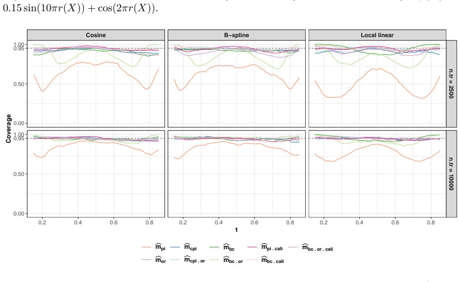
- [§4.2.2 and Figure 5] The coverage analysis targets the smoothed estimand rather than m(t) (or τ(t)); the application's confidence bands should state explicitly whether they target the smoothed version or the true curve. Currently Figure 5's caption just says '95% confidence band'.
- [References] Some references are preprints with future dates (e.g., Zhang et al. 2026, Tian et al. 2026). Please add 'arXiv' identifiers or publication status to avoid ambiguity.
Circularity Check
No circularity: the central rate claims are conditional upper bounds, not predictions forced by construction.
full rationale
No circularity found. The proposed estimators are constructed from explicit influence functions and direct bias-correction decompositions (Sections 2.1-2.2, 3.1-3.2), and the rate results in Propositions 1-4 are stated as upper bounds depending on the first-stage error norm \|\hat r-r\|, not on the target m(t). The key conditions Assumptions 2, 3, 7, and 8 are explicitly stated as assumptions; the paper does not claim they follow from the maintained condition E(\rho|r)=0, and it repeatedly flags that if Assumption 3/8 fails the nuisance bias is only first-order in \|\hat r-r\|, rendering the debiasing ineffective. That dependency is a correctness/robustness concern, not a circular reduction. The self-citations (Kennedy 2022, 2023; Bonvini & Kennedy 2022) are used as general semiparametric tools and do not encode the paper's target rates; no uniqueness theorem is imported to force the estimator choice. The simulation studies and the NLSY97 application provide external checks, and the empirical finding is an estimated effect consistent with prior literature rather than a quantity fitted to produce that conclusion. Thus the derivation chain is self-contained and no circular step can be exhibited.
Axiom & Free-Parameter Ledger
free parameters (5)
- Second-stage bandwidth h (local linear estimators)
- Derivative-estimation bandwidth b (lcpi)
- Sieve dimension k (sbc/scpi)
- Sieve dimension q for derivative (scpi)
- First-stage nuisance tuning parameters (Lasso lambda, stacking weights, random forest hyperparameters)
axioms (8)
- domain assumption Assumption 1: r(X) is continuously distributed on a compact interval with density bounded above and away from zero; m is twice differentiable with bounded derivatives; Y and A are bounded.
- domain assumption Sample splitting: \hat{r} and \hat{\mu} are estimated on a separate auxiliary sample D_n, independent of the second-stage sample.
- domain assumption First-stage accuracy relative to smoothing scale: ||\hat{r}-r||_\infty=o(h) for local smoothing and o(1/k) for sieves.
- domain assumption Assumptions 2 and 7: ||\hat{\mu}-\mu||_\infty \lesssim ||\hat{r}-r||_\infty and related L2 product bounds.
- domain assumption Assumptions 3 and 8: |E(\rho|\hat{r}=t_1, r=t_2, D_n)| \lesssim ||\hat{r}-r||_\infty and corresponding L2 bounds on E(\rho|\hat{r},r,D_n).
- standard math Assumptions 4, 5, 6: sieve Gram matrices Q_{\Phi,k}(r), Q_{\dot{\Phi},k}(r) are well-conditioned uniformly in k; cosine-basis norm bounds \xi_k \lesssim \sqrt{k}, \eta_k \lesssim k^{3/2}, \zeta_k \lesssim k^{5/2}.
- standard math Assumption 9: approximation error ||\Delta_k||_\infty \lesssim k^{-s} for a H\"older-smooth m.
- ad hoc to paper Application identifiability and pseudo-outcome transfer: no unmeasured confounding, positivity, consistency; the estimated DR pseudo-outcome \hat{\phi}(Z) has second-order errors so Propositions 1-4 continue to hold.
Cite this review
Pith. "Pith review of On regression with estimated covariates and conditional effects given the propensity score." pith.science (2026). https://pith.science/paper/HK4UM653
@misc{pith2026260727685,
  author       = {Pith},
  title        = {Pith review of: On regression with estimated covariates and conditional effects given the propensity score},
  year         = {2026},
  howpublished = {\url{https://pith.science/paper/HK4UM653}},
  note         = {Machine review of arXiv:2607.27685}
}
read the original abstract
Motivated by the study of heterogeneous returns to education in Brand & Xie 2010, which considers how the effect of completing college on earnings varies with the (unknown) probability of completing college, we analyze the problem of estimating a nonparametric regression function when certain covariates are estimated in a first step. Plug-in estimators that treat the estimated covariates as known generally suffer from first-stage estimation error. To mitigate this issue, we analyze two debiasing approaches within a framework that is agnostic to the choice of the first-stage estimation method and relies on either local-smoothing or sieve-based methods for the second-stage regression. In particular, we consider: (i) influence function-based estimators of pathwise differentiable parameters that approximate the target estimand, and (ii) a variant of plug-in estimators that directly aims to correct their bias. For each method, we upper bound the estimation error and characterize conditions under which oracle rates can be approached, highlighting the possible gains in terms of convergence rates relative to the plug-ins. Simulation studies illustrate the finite-sample behavior of the methods. We apply our methodology to data from the National Longitudinal Survey of Youth 1997 and find evidence that completing college yields the largest reductions in unemployment for individuals least likely to do so, consistent with earlier findings in the literature (Brand & Xie 2010; Brand 2023).
Figures




Reference graph
Works this paper leans on
-
[1]
Andrews, D. W. Nonparametric kernel estimation for semiparametric models.Econometric Theory11,560–586 (1995)
1995
-
[2]
& Kato, K
Belloni, A., Chernozhukov, V., Chetverikov, D. & Kato, K. Some new asymptotic theory for least squares series: Pointwise and uniform results.Journal of Econometrics186,345–366 (2015)
2015
-
[3]
A., Ritov, Y
Bickel, P., Klaassen, C. A., Ritov, Y. & Wellner, J. A.Efficient and adaptive estimation for semiparametric models(Springer-Verlag New York, 1993)
1993
-
[4]
Bonvini, M. & Kennedy, E. H. Fast convergence rates for dose-response estimation.arXiv preprint arXiv:2207.11825(2022)
Pith/arXiv arXiv 2022
-
[5]
E.Overcoming the odds: The benefits of completing college for unlikely graduates (Russell Sage Foundation, 2023)
Brand, J. E.Overcoming the odds: The benefits of completing college for unlikely graduates (Russell Sage Foundation, 2023)
2023
-
[6]
Brand, J. E. & Xie, Y. Who benefits most from college? Evidence for negative selection in heterogeneous economic returns to higher education.American sociological review75,273– 302 (2010)
2010
-
[7]
Calonico, S., Cattaneo, M. D. & Farrell, M. H. nprobust: Nonparametric kernel-based estima- tion and robust bias-corrected inference.arXiv preprint arXiv:1906.00198(2019)
Pith/arXiv arXiv 1906
-
[8]
& Robins, J
Chernozhukov, V., Chetverikov, D., Demirer, M., Duflo, E., Hansen, C., Newey, W. & Robins, J. Double/debiased machine learning for treatment and structural parameters.The Econo- metrics Journal21,C1–C68 (2018)
2018
-
[9]
Chernozhukov, V., Newey, W. K., Quintas-Martinez, V. & Syrgkanis, V. Automatic debiased machine learning via riesz regression.arXiv preprint arXiv:2104.14737(2021)
Pith/arXiv arXiv 2021
-
[10]
C., Jacho-Ch´ avez, D
Escanciano, J. C., Jacho-Ch´ avez, D. T. & Lewbel, A. Uniform convergence of weighted sums of non and semiparametric residuals for estimation and testing.Journal of Econometrics178, 426–443 (2014)
2014
-
[11]
Escanciano, J. C. & P´ erez-Izquierdo, T. Automatic Locally Robust Estimation with Generated Regressors.arXiv preprint arXiv:2301.10643(2023)
arXiv 2023
-
[12]
& Truong, Y
Fan, J. & Truong, Y. K. Nonparametric regression with errors in variables.The Annals of Statistics,1900–1925 (1993)
1900
-
[13]
Foster, D. J. & Syrgkanis, V. Orthogonal statistical learning.The Annals of Statistics51, 879–908 (2023)
2023
-
[14]
& Ridder, G
Hahn, J., Liao, Z. & Ridder, G. Nonparametric two-step sieve M estimation and inference. Econometric Theory34,1281–1324 (2018)
2018
-
[15]
& Ridder, G
Hahn, J. & Ridder, G. Asymptotic variance of semiparametric estimators with generated regressors.Econometrica81,315–340 (2013)
2013
-
[16]
Imbens, G. W. & Rubin, D. B.Causal inference in statistics, social, and biomedical sciences (Cambridge University Press, 2015)
2015
-
[17]
Kennedy, E. H. Semiparametric doubly robust targeted double machine learning: a review. arXiv preprint arXiv:2203.06469(2022). 29
Pith/arXiv arXiv 2022
-
[18]
Kennedy, E. H. Towards optimal doubly robust estimation of heterogeneous causal effects. Electronic Journal of Statistics17,3008–3049 (2023)
2023
-
[19]
H., Balakrishnan, S., Robins, J
Kennedy, E. H., Balakrishnan, S., Robins, J. M. & Wasserman, L. Minimax rates for hetero- geneous causal effect estimation.arXiv preprint arXiv:2203.00837(2022)
Pith/arXiv arXiv 2022
-
[20]
H., Ma, Z., McHugh, M
Kennedy, E. H., Ma, Z., McHugh, M. D. & Small, D. S. Nonparametric methods for doubly robust estimation of continuous treatment effects.Journal of the Royal Statistical Society. Series B, Statistical Methodology79,1229 (2017)
2017
-
[21]
Liu, L., Mukherjee, R., Newey, W. K. & Robins, J. M. Semiparametric efficient empirical higher order influence function estimators.arXiv preprint arXiv:1705.07577(2017)
arXiv 2017
-
[22]
& Chung, I
Luedtke, A. & Chung, I. One-step estimation of differentiable hilbert-valued parameters.The Annals of Statistics52,1534–1563 (2024)
2024
-
[23]
& Schienle, M
Mammen, E., Rothe, C. & Schienle, M. Nonparametric regression with nonparametrically generated covariates.The Annals of Statistics40,1132–1170 (2012)
2012
-
[24]
& Schienle, M
Mammen, E., Rothe, C. & Schienle, M. Semiparametric estimation with generated covariates. Econometric Theory32,1140–1177 (2016)
2016
-
[25]
& Mukherjee, R
McGrath, S. & Mukherjee, R. Nuisance Function Tuning and Sample Splitting for Optimally Estimating a Doubly Robust Functional.Annals of statistics(2026)
2026
-
[26]
& Wager, S
Nie, X. & Wager, S. Quasi-oracle estimation of heterogeneous treatment effects.Biometrika 108,299–319 (2021)
2021
-
[27]
Robins, J., Li, L., Mukherjee, R., Tchetgen, E. T. & van der Vaart, A. Higher order estimating equations for high-dimensional models.Annals of statistics45,1951 (2017)
1951
-
[28]
M., Rotnitzky, A
Robins, J. M., Rotnitzky, A. & Zhao, L. P. Estimation of regression coefficients when some regressors are not always observed.Journal of the American statistical Association89,846– 866 (1994)
1994
-
[29]
& Nielsen, J
Scholz, M., Sperlich, S. & Nielsen, J. P. Nonparametric long term prediction of stock returns with generated bond yields.Insurance: Mathematics and Economics69,82–96 (2016)
2016
-
[30]
& Chernozhukov, V
Semenova, V. & Chernozhukov, V. Debiased machine learning of conditional average treatment effects and other causal functions.The Econometrics Journal24,264–289 (2021)
2021
-
[31]
Uniform convergence of series estimators over function spaces.Econometric Theory 24,1463–1499 (2008)
Song, K. Uniform convergence of series estimators over function spaces.Econometric Theory 24,1463–1499 (2008)
2008
-
[32]
A note on non-parametric estimation with predicted variables.The Econometrics Journal12,382–395 (2009)
Sperlich, S. A note on non-parametric estimation with predicted variables.The Econometrics Journal12,382–395 (2009)
2009
-
[33]
Tian, P., Yang, F. & Ding, P. Bracketing Relationships of Weighted Average Treatment Effects. arXiv preprint arXiv:2606.11715(2026)
Pith/arXiv arXiv 2026
-
[34]
A.Semiparametric theory and missing data(Springer Science & Business Media, 2006)
Tsiatis, A. A.Semiparametric theory and missing data(Springer Science & Business Media, 2006)
2006
-
[35]
B.Introduction to nonparametric estimation(Springer Science & Business Me- dia, 2008)
Tsybakov, A. B.Introduction to nonparametric estimation(Springer Science & Business Me- dia, 2008)
2008
-
[36]
Van der Laan, L., Luedtke, A. & Carone, M. Automatic doubly robust inference for linear functionals via calibrated debiased machine learning.arXiv preprint arXiv:2411.02771(2024)
Pith/arXiv arXiv 2024
-
[37]
(Cambridge University Press, Cambridge, 2026)
Vershynin, R.High-Dimensional Probability: An Introduction with Applications in Data Sci- ence2nd ed. (Cambridge University Press, Cambridge, 2026)
2026
-
[38]
Wu, P., Han, S., Tong, X. & Li, R. Propensity Score Regression for Causal Inference with Treatment Heterogeneity.Statistica Sinica34,747–769. doi:10 . 5705 / ss . 202022 . 0008. https://doi.org/10.5705/ss.202022.0008(2024)
arXiv 2024
-
[39]
Xie, Y., Brand, J. E. & Jann, B. Estimating heterogeneous treatment effects with observational data.Sociological methodology42,314–347 (2012). 30
2012
-
[40]
Zhang, Y., Liu, L. & Zhang, Z. Higher-Order Debiased Estimators for General Treatment Models.arXiv preprint arXiv:2606.01706(2026). 31 A Estimated outcomes versus estimated covariates At the surface level, the problem of estimating a regression function with unobserved, but estimable, covariates resembles that of estimating a regression with an unobserved...
Pith/arXiv arXiv 2026
This paper was first reviewed by deepseek-v4-flash on August 1, 2026.
discussion (0)
Sign in with ORCID, Apple, or X to comment. Anyone can read and Pith papers without signing in.