REVIEW 4 major objections 5 minor 44 references
BPQP: A Differentiable Convex Optimization Framework for Efficient End-to-End Learning
T0 review · 4 major / 5 minor · reviewed 2026-08-12 · deepseek-v4-flash
Pith's one-line read The paper claims that the backward pass through a differentiable convex optimization layer can be rewritten as an equality-constrained quadratic program, making gradient computation a standard QP solve.
desk verdict A genuinely useful reformulation of the backward pass as an equality-constrained QP, with a correct-but-underspecified Theorem 1 and a strong but slightly messy experimental section. read the letter →
The pith
A machine-rendered reading of the paper's core claim, the machinery that carries it, and where it could break.
The reading
What carries the argument
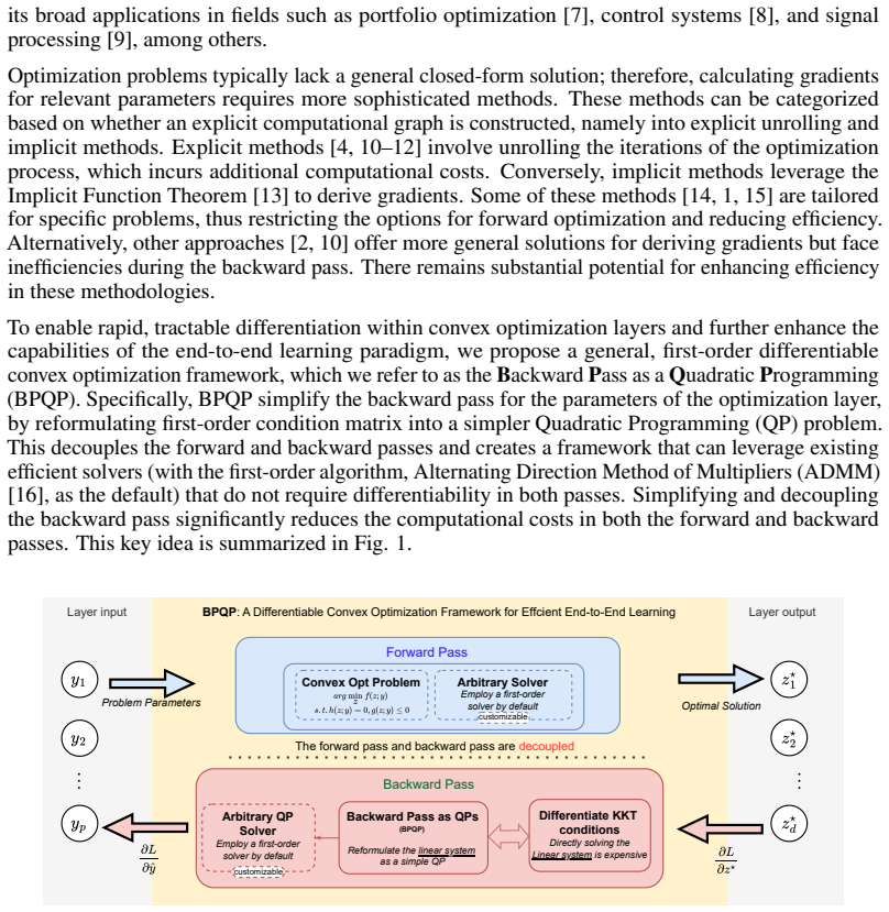
The central object is the KKT matrix of the forward optimization problem, and the key move is to replace its complementarity block — the diagonal matrices $D(\lambda^\star)G(z^\star)$ and $D(g(z^\star))$ — with equality constraints on the active set, the set of inequality constraints that hold with equality at the optimum. Because the active set is known after the forward pass, the backward gradient vector solves the equality-constrained quadratic program in Eq. (6), whose KKT conditions reproduce the desired linear system exactly. This hands the backward pass to any QP solver; the paper uses a first-order ADMM solver with sparsity, solution polishing, and active-set machinery, plus a small regularization $\delta I$ to handle redundant constraints.
What would settle it
Construct a small QP whose optimum has an inequality constraint with a dual multiplier comparable to the solver's tolerance (for example $10^{-6}$), then compute the backward gradient both by the paper's Eq. (6) and by a high-precision solution of Eq. (3). If the two disagree beyond numerical noise, or if changing the solver tolerance flips the active set and produces a discontinuous gradient, the exact-equivalence premise of Theorem 1 fails in a practically reachable regime.
Extended reading notes
Core claim
The central claim is Theorem 1. Once the forward pass has identified the active set of inequality constraints, the vector $[\tilde z, \tilde\lambda, \tilde\nu]$ that solves the backward KKT system (Eq. 3) is exactly the optimal solution of the equality-constrained quadratic program (Eq. 6) with objective $\tfrac12 \tilde z^\top P' \tilde z + q'^\top \tilde z$ and constraints $A'\tilde z = b'$, $G'_+\tilde z = c'_+$. The complementarity block of the KKT matrix is replaced by the active-set equality rows, which turns the backward system into a plain convex QP that any QP solver can handle. To guard against a singular KKT matrix, the implementation adds a small regularization to the diagonal. On simulated problems the resulting gradients match a high-precision KKT solve with 0.992 cosine similarity for QP, while total runtime is reduced by up to 21x on LP layers.
Load-bearing premise
The equivalence in Theorem 1 rests on knowing the exact active set and on every active inequality having a strictly positive dual multiplier; a first-order solver returns only a finite-tolerance solution, so on weakly active or degenerate constraints the active set is approximate and the backward QP can return a different gradient from the exact KKT system.
Editorial extensions
If this is right
- End-to-end training of networks with optimization layers becomes practical at problem scales where direct KKT inversion is prohibitively slow, such as the reported 500-asset portfolio optimization task.
- Because the backward pass is a standard convex QP, future improvements in QP solvers translate directly into faster differentiable layers without changing the method.
- The forward solver no longer needs to be differentiable or share factorizations with the backward pass, so each pass can use the best available algorithm for its structure.
- The paper's measurements show total runtime speedups of up to 13.54x on quadratic programs, 21.02x on linear programs, and 1.67x on second-order cone programs, with backward gradient cosine similarity 0.992 on QP against a high-precision KKT solve.
- The method scales to large sparse problems (up to 5000x2000 in the experiments), where the paper reports that competing differentiable layers fail to generate results.
Reading between the lines
- Inference: the reported speedups should grow with the fraction of inactive constraints, since the backward QP keeps only the active rows; the paper does not isolate this dependence, but it follows directly from the reformulation.
- Inference: because the active set is read off a finite-tolerance solver's output, the natural stress test is a degenerate problem where a dual multiplier is near zero; Theorem 1 is stated without explicitly requiring strictly positive multipliers on all active inequalities, and this is where the backward QP gradient could diverge from the exact KKT value.
- Inference: the same active-set-to-QP trick could be applied to higher-order derivative computations, such as Hessian-vector products, or to non-convex forward maps near a local minimum, since the derivation only uses the KKT structure at the returned point; the paper hints at the non-convex extension but does not test it.
Editorial analysis
A structured set of objections, weighed in public.
Referee Report
Summary. The paper proposes BPQP, a differentiable convex optimization layer that reformulates the backward pass of implicit differentiation as an equality-constrained quadratic program (Eq. 6) whose KKT system coincides with the linear system obtained by differentiating the KKT conditions of the forward problem (Eq. 3), under an active-set replacement. The backward QP is then solved with OSQP, decoupling the forward and backward solvers. Experiments compare runtime and gradient accuracy against CVXPY, qpth/OptNet, Alt-Diff, JAXOpt, and an Exact matrix-inverse baseline on randomly generated QPs, LPs, and SOCPs, and on a CSI 500 portfolio-optimization task, reporting large speedups and competitive or improved decision metrics.
Significance. If the equivalence in Theorem 1 is established under the right assumptions, the central idea is practically useful: it turns the backward linear solve into a convex QP that can leverage mature first-order solvers, and the decoupling of forward and backward passes is attractive for large-scale end-to-end learning. The paper provides a proof in Appendix A.2, releases code through Qlib, and reports extensive runtime and accuracy experiments. Its value, however, depends on the exactness of the backward gradient under the stated conditions, which are currently too weak, and on the credibility of the LP and SOCP experimental claims. The theoretical contribution is a reformulation with empirical support rather than a new mathematical theory.
major comments (4)
- [Theorem 1 / Appendix A.2] The proof of Theorem 1 replaces the complementarity block D(λ*)G(z*) and D(g(z*)) in Eq. (3) with the equality block G_+ in Eqs. (20)-(21). This replacement is exact only when the active set is known exactly and every active inequality satisfies λ*_i > 0 (strict complementarity). The stated assumptions—'not primal infeasible' and 'the corresponding Jacobian vector ∇yL exists'—do not imply strict complementarity. When a constraint is weakly active (g_i(z*)=0, λ*_i=0), the i-th complementarity row of Eq. (3) is identically 0=0 and imposes no constraint on \tilde z, while Eq. (6) enforces G_{i+}\tilde z=0; the two systems can then produce different gradients. A concrete degenerate case is min_z 0.5||z||^2 + q^T z subject to z_i ≤ 0 at q=0 with loss L=z_1+z_2, where Eq. (3) admits both \tilde z=(-1,-1) and \tilde z=(0,0), but Eq. (6) forces \tilde z=0. In addition, OSQP returns solutions only to finite tolerance (Section 4.2), so the active set recovered from the forward pass is approximate; a near-active constraint that is misclassified changes Eq. (6) and hence the gradient. Theorem 1 should state the strict-complementarity and exact-active-set assumptions, or be reformulated as an approximate-gradient statement with a perturbation bound.
- [Section 5.1, Eq. (17)] The experiments labeled 'LP' solve minimize θ^T z + ε||z||^2_2 subject to Az=b, Gz≤h with ε=10^{-6}. This is a strictly convex quadratic program, not a linear program. For a genuine LP (P=0), the KKT matrix in Eq. (3) can be singular and the backward solution nonunique; the paper provides no analysis of this case. Consequently, the claimed 21.02× speedup on LP and the statement that BPQP handles LP layers are not demonstrated for standard LPs. The experiment should be reported as 'regularized LP' or, preferably, true LP instances should be tested with a discussion of degeneracy and uniqueness.
- [Table 1] Table 1 gives absolute times with row labels '(scale 1.0e-04)' for Exact, CVXPY, qpth/OptNet, Alt-Diff, and JAXOpt, but '(scale 1.0e+00)' for BPQP. As printed, the BPQP entries are in different units from the other entries, and the quoted speedups in the abstract and Section 1 are not recoverable unless all rows are read with the same implicit scale. For example, the QP 100×20 total time for Exact is 484.2×10^{-4} s and for BPQP is 35.1×10^{-4} s if the same scale is used, giving the ~13.5× speedup; with the printed scale labels, BPQP would appear to be orders of magnitude slower. Please restate the table with one explicit unit for all rows or report raw times in a common unit.
- [Section 6 and 'General Gradients' in Section 4.1] The claim that BPQP 'is still equipped to reformulate the backward pass as a QP' for non-convex problems is not supported. For a non-convex objective, the matrix P' in Eq. (6) need not be positive semidefinite, so the backward problem is not a convex QP and OSQP's convergence guarantees (Section 4.2) do not apply. The 'General Gradients' paragraph defines gradients that preserve the KKT norm at intermediate iterates, but Appendix A.4 does not show that these surrogate vectors equal or approximate the true loss gradient; it only states an identity dr(k)=0 and concludes norm preservation. This is a heuristic, not a theorem. Either provide conditions under which the KKT-norm-preserving update yields the correct gradient, or remove the non-convex claims from the discussion.
minor comments (5)
- [Definition 1 and Section 3.2] There are dimension errors in the notation: h should map R^d to R^m and g should map R^d to R^n, and the backward variables in Eq. (3) should be \tilde λ ∈ R^n and \tilde ν ∈ R^m, not the reverse as printed.
- [Section 4.1] The condition list for equivalence of Eq. (5) and Eq. (3) is confusing: D(\tilde λ)G' = D(λ*)G(z*) is a matrix equation involving the unknown \tilde λ, not a condition that can be checked a priori. The exposition would benefit from stating that the active-set replacement is used precisely to avoid this issue.
- [Appendix A.2, Eq. (19)] There is a typo: 'the original optimization problem in can be reformulated' should read 'in Definition 1 can be reformulated'.
- [Table 3] The text says 'The CosSim. of all methods are small enough for SOCP' but the table shows values of 1.00; the intended wording is probably 'close to one' or 'sufficiently high'.
- [Section 6] The sentence 'While its hard to perform experiments on non-convex problem due to the lack of baselines' contains grammar errors and should be rephrased.
Circularity Check
No significant circularity: BPQP's backward QP reformulation is a mathematical equivalence, not a refit or self-citation reduction.
full rationale
The load-bearing step is Theorem 1 and Appendix A.2: Eq. (21) is obtained by replacing the complementarity block D(lambda*)G(z*) with G+(z*) after restricting to the active set, and Eq. (22) is exactly the KKT system of the equality-constrained QP (6). This is an algebraic equivalence between two linear systems, with no fitted parameter entering the gradient formula. P', A', G'_+, q', c'_+, and b' are taken directly from the forward-pass KKT data and the given loss gradient; no term is tuned to reproduce the target gradient. The added regularizers delta and epsilon are fixed constants (10^-6) and are not calibrated against the quantities being predicted. The QP/LP/SOCP speedups and portfolio results are benchmarked against external baselines (OptNet, CVXPY, JAXOpt, Alt-Diff, Exact, Two-Stage), so they do not reduce to the paper's own assumptions. The active-set replacement in Eq. (20) can fail under weak complementarity or finite OSQP tolerance, but that is a correctness/robustness concern about the assumption, not a circularity: the derivation does not define the gradient in terms of itself. The 'General Gradients' paragraph is under-specified but is not used to fit any parameter or to produce the reported results. No load-bearing self-citation was found; [24] is a code release and [14,16] are external prior work. Therefore the derivation is self-contained with respect to circularity.
Assumptions & free parameters
free parameters (5)
- LP regularization epsilon =
1e-6
- KKT regularization delta =
1e-6
- OSQP termination tolerances =
abs/rel tolerance 1e-3, max iterations 4000 (simulated); 1e-5 (portfolio)
- Portfolio loss weight beta =
0.1
- Risk aversion coefficient gamma =
1
assumptions (4)
- domain assumption The convex optimization layer satisfies KKT necessity (a constraint qualification such as Slater or LICQ) and the KKT matrix is invertible at the optimum.
- ad hoc to paper The active set is correctly identified from the forward solution and strict complementarity holds for active constraints, so replacing inequalities with equalities in Eq. (20) preserves the linear system solution.
- standard math OSQP's ADMM with iterative refinement converges to the exact solution of the regularized KKT system in practice, with one backward and one forward solve as in Eq. (11).
- domain assumption The Hessian of the Lagrangian P(z*,nu*,lambda*) is positive semidefinite for the problem classes considered, so the backward QP is convex.
Cite this review
Pith. "Pith review of BPQP: A Differentiable Convex Optimization Framework for Efficient End-to-End Learning." pith.science (2026). https://pith.science/paper/HRNCYU3O
@misc{pith2026241119285,
  author       = {Pith},
  title        = {Pith review of: BPQP: A Differentiable Convex Optimization Framework for Efficient End-to-End Learning},
  year         = {2026},
  howpublished = {\url{https://pith.science/paper/HRNCYU3O}},
  note         = {Machine review of arXiv:2411.19285}
}
read the original abstract
Data-driven decision-making processes increasingly utilize end-to-end learnable deep neural networks to render final decisions. Sometimes, the output of the forward functions in certain layers is determined by the solutions to mathematical optimization problems, leading to the emergence of differentiable optimization layers that permit gradient back-propagation. However, real-world scenarios often involve large-scale datasets and numerous constraints, presenting significant challenges. Current methods for differentiating optimization problems typically rely on implicit differentiation, which necessitates costly computations on the Jacobian matrices, resulting in low efficiency. In this paper, we introduce BPQP, a differentiable convex optimization framework designed for efficient end-to-end learning. To enhance efficiency, we reformulate the backward pass as a simplified and decoupled quadratic programming problem by leveraging the structural properties of the KKT matrix. This reformulation enables the use of first-order optimization algorithms in calculating the backward pass gradients, allowing our framework to potentially utilize any state-of-the-art solver. As solver technologies evolve, BPQP can continuously adapt and improve its efficiency. Extensive experiments on both simulated and real-world datasets demonstrate that BPQP achieves a significant improvement in efficiency--typically an order of magnitude faster in overall execution time compared to other differentiable optimization layers. Our results not only highlight the efficiency gains of BPQP but also underscore its superiority over differentiable optimization layer baselines.
Figures


Reference graph
Works this paper leans on
-
[1]
Differentiable convex optimization layers
Akshay Agrawal, Brandon Amos, Shane Barratt, Stephen Boyd, Steven Diamond, and J Zico Kolter. Differentiable convex optimization layers. Advances in neural information processing 10 systems, 32, 2019
work page 2019
-
[2]
Stephen Gould, Richard Hartley, and Dylan Campbell. Deep declarative networks. IEEE Transactions on Pattern Analysis and Machine Intelligence, 44(8):3988–4004, 2021
work page 2021
-
[3]
A tutorial on energy- based learning
Yann LeCun, Sumit Chopra, Raia Hadsell, M Ranzato, and Fujie Huang. A tutorial on energy- based learning. Predicting structured data, 1(0), 2006
2006
-
[4]
Generic methods for optimization-based modeling
Justin Domke. Generic methods for optimization-based modeling. In Artificial Intelligence and Statistics, pages 318–326. PMLR, 2012
work page 2012
-
[5]
Smart predict-and-optimize for hard combina- torial optimization problems
Jayanta Mandi, Peter J Stuckey, Tias Guns, et al. Smart predict-and-optimize for hard combina- torial optimization problems. In Proceedings of the AAAI Conference on Artificial Intelligence, volume 34, pages 1603–1610, 2020
work page 2020
-
[6]
predict, then optimize
Adam N Elmachtoub and Paul Grigas. Smart “predict, then optimize”. Management Science, 68(1):9–26, 2022
2022
-
[7]
Melding the data-decisions pipeline: Decision- focused learning for combinatorial optimization
Bryan Wilder, Bistra Dilkina, and Milind Tambe. Melding the data-decisions pipeline: Decision- focused learning for combinatorial optimization. In Proceedings of the AAAI Conference on Artificial Intelligence, volume 33, pages 1658–1665, 2019
work page 2019
-
[8]
Stochastic distribution control system design: a convex optimization approach
Lei Guo and Hong Wang. Stochastic distribution control system design: a convex optimization approach. Springer, 2010
work page 2010
Show all 44 references
-
[9]
Real-time convex optimization in signal processing
John Mattingley and Stephen Boyd. Real-time convex optimization in signal processing. IEEE Signal Processing Magazine, 27(3):50–61, 2010
2010
-
[10]
Efficient and modular implicit differentiation
Mathieu Blondel, Quentin Berthet, Marco Cuturi, Roy Frostig, Stephan Hoyer, Felipe Llinares- López, Fabian Pedregosa, and Jean-Philippe Vert. Efficient and modular implicit differentiation. arXiv preprint arXiv:2105.15183, 2021
2021 arXiv
-
[11]
Efficient multiple hyperparameter learning for log-linear models
Chuan-sheng Foo, Andrew Ng, et al. Efficient multiple hyperparameter learning for log-linear models. In Advances in neural information processing systems, volume 20, 2007
2007
-
[12]
Alternating differentiation for optimization layers
Haixiang Sun, Ye Shi, Jingya Wang, Hoang Duong Tuan, H Vincent Poor, and Dacheng Tao. Alternating differentiation for optimization layers. In The Eleventh International Conference on Learning Representations, 2022
2022
-
[13]
An implicit function theorem
K Jittorntrum. An implicit function theorem. Journal of Optimization Theory and Applications, 25(4):575–577, 1978
1978
-
[14]
Optnet: Differentiable optimization as a layer in neural networks
Brandon Amos and J Zico Kolter. Optnet: Differentiable optimization as a layer in neural networks. In International Conference on Machine Learning, pages 136–145. PMLR, 2017
2017
-
[15]
Differenti- ating through a cone program
Akshay Agrawal, Shane Barratt, Stephen Boyd, Enzo Busseti, and Walaa M Moursi. Differenti- ating through a cone program. arXiv preprint arXiv:1904.09043, 2019
1904 arXiv
-
[16]
Osqp: An operator splitting solver for quadratic programs
Bartolomeo Stellato, Goran Banjac, Paul Goulart, Alberto Bemporad, and Stephen Boyd. Osqp: An operator splitting solver for quadratic programs. Mathematical Programming Computation, 12(4):637–672, 2020
2020
-
[17]
The simplex method for quadratic programming
Philip Wolfe. The simplex method for quadratic programming. Econometrica: Journal of the Econometric Society, pages 382–398, 1959
1959
-
[18]
Efficient differentiable quadratic programming layers: an admm approach
Andrew Butler and Roy H Kwon. Efficient differentiable quadratic programming layers: an admm approach. Computational Optimization and Applications, 84(2):449–476, 2023
2023
-
[19]
Cvxpy: A python-embedded modeling language for convex optimization
Steven Diamond and Stephen Boyd. Cvxpy: A python-embedded modeling language for convex optimization. The Journal of Machine Learning Research, 17(1):2909–2913, 2016
2016
-
[20]
Conic optimization via operator splitting and homogeneous self-dual embedding
Brendan O’donoghue, Eric Chu, Neal Parikh, and Stephen Boyd. Conic optimization via operator splitting and homogeneous self-dual embedding. Journal of Optimization Theory and Applications, 169:1042–1068, 2016. 11
2016
-
[21]
Mipaal: Mixed integer program as a layer
Aaron Ferber, Bryan Wilder, Bistra Dilkina, and Milind Tambe. Mipaal: Mixed integer program as a layer. In Proceedings of the AAAI Conference on Artificial Intelligence, volume 34, pages 1504–1511, 2020
2020
-
[22]
Implicit mle: backpropagating through discrete exponential family distributions
Mathias Niepert, Pasquale Minervini, and Luca Franceschi. Implicit mle: backpropagating through discrete exponential family distributions. InAdvances in Neural Information Processing Systems, 2021
2021
-
[23]
Satnet: Bridging deep learning and logical reasoning using a differentiable satisfiability solver
Po-Wei Wang, Priya Donti, Bryan Wilder, and Zico Kolter. Satnet: Bridging deep learning and logical reasoning using a differentiable satisfiability solver. In International Conference on Machine Learning, pages 6545–6554. PMLR, 2019
2019
-
[24]
Qlib: An ai-oriented quantitative investment platform
Xiao Yang, Weiqing Liu, Dong Zhou, Jiang Bian, and Tie-Yan Liu. Qlib: An ai-oriented quantitative investment platform. arXiv preprint arXiv:2009.11189, 2020
2009 arXiv
-
[25]
Robust linear programming discrimination of two linearly inseparable sets
Kristin P Bennett and Olvi L Mangasarian. Robust linear programming discrimination of two linearly inseparable sets. Optimization methods and software, 1(1):23–34, 1992
1992
-
[26]
End-to-end risk budgeting portfolio optimiza- tion with neural networks
A Sinem Uysal, Xiaoyue Li, and John M Mulvey. End-to-end risk budgeting portfolio optimiza- tion with neural networks. Annals of Operations Research, pages 1–30, 2023
2023
-
[27]
H. M. Markowitz. Portfolio selection. The journal of finance, 7(1):77–91, 1952
1952
-
[28]
V olatility clustering in financial markets: a microsimulation of interacting agents
Thomas Lux and Michele Marchesi. V olatility clustering in financial markets: a microsimulation of interacting agents. International journal of theoretical and applied finance, 3(04):675–702, 2000
2000
-
[29]
Improved svrg for non-strongly-convex or sum-of-non- convex objectives
Zeyuan Allen-Zhu and Yang Yuan. Improved svrg for non-strongly-convex or sum-of-non- convex objectives. In International conference on machine learning, pages 1080–1089. PMLR, 2016
2016
-
[30]
Dc3: A learning method for optimization with hard constraints
Priya L Donti, David Rolnick, and J Zico Kolter. Dc3: A learning method for optimization with hard constraints. arXiv preprint arXiv:2104.12225, 2021
2021 arXiv
-
[31]
End-to-end learning for optimization via constraint-enforcing approximators
Rares Cristian, Pavithra Harsha, Georgia Perakis, Brian L Quanz, and Ioannis Spantidakis. End-to-end learning for optimization via constraint-enforcing approximators. In Proceedings of the AAAI Conference on Artificial Intelligence, volume 37, pages 7253–7260, 2023
2023
-
[32]
End-to-end stochastic optimization with energy-based model
Lingkai Kong, Jiaming Cui, Yuchen Zhuang, Rui Feng, B Aditya Prakash, and Chao Zhang. End-to-end stochastic optimization with energy-based model. Advances in Neural Information Processing Systems, 35:11341–11354, 2022
2022
-
[33]
Learning the travelling salesperson problem requires rethinking generalization
Chaitanya K Joshi, Quentin Cappart, Louis-Martin Rousseau, and Thomas Laurent. Learning the travelling salesperson problem requires rethinking generalization. Constraints, pages 1–29, 2022
2022
-
[34]
Learning combinatorial optimization algorithms over graphs
Elias Khalil, Hanjun Dai, Yuyu Zhang, Bistra Dilkina, and Le Song. Learning combinatorial optimization algorithms over graphs. Advances in neural information processing systems, 30, 2017
2017
-
[35]
Combinatorial opti- mization by graph pointer networks and hierarchical reinforcement learning
Qiang Ma, Suwen Ge, Danyang He, Darshan Thaker, and Iddo Drori. Combinatorial opti- mization by graph pointer networks and hierarchical reinforcement learning. arXiv preprint arXiv:1911.04936, 2019
1911 arXiv
-
[36]
Attention, learn to solve routing problems! arXiv preprint arXiv:1803.08475, 2018
Wouter Kool, Herke Van Hoof, and Max Welling. Attention, learn to solve routing problems! arXiv preprint arXiv:1803.08475, 2018
2018 arXiv
-
[37]
End-to-end risk budgeting portfolio optimization with neural networks
Ayse Sinem Uysal, Xiaoyue Li, and John M Mulvey. End-to-end risk budgeting portfolio optimization with neural networks. arXiv preprint arXiv:2107.04636, 2021
2021 arXiv
-
[38]
Decision-focused learning without differentiable optimization: Learning locally optimized decision losses
Sanket Shah, Kai Wang, Bryan Wilder, Andrew Perrault, and Milind Tambe. Decision-focused learning without differentiable optimization: Learning locally optimized decision losses. arXiv preprint arXiv:2203.16067, 2022. 12
2022 arXiv
-
[39]
Automatically learning compact quality-aware surrogates for optimization problems
Kai Wang, Bryan Wilder, Andrew Perrault, and Milind Tambe. Automatically learning compact quality-aware surrogates for optimization problems. Advances in Neural Information Processing Systems, 33:9586–9596, 2020
2020
-
[40]
Surco: Learning linear surrogates for combinatorial nonlinear optimization problems
Aaron M Ferber, Taoan Huang, Daochen Zha, Martin Schubert, Benoit Steiner, Bistra Dilkina, and Yuandong Tian. Surco: Learning linear surrogates for combinatorial nonlinear optimization problems. In International Conference on Machine Learning , pages 10034–10052. PMLR, 2023
2023
-
[41]
Landscape surrogate: Learning decision losses for mathematical optimization under partial information
Arman Zharmagambetov, Brandon Amos, Aaron Ferber, Taoan Huang, Bistra Dilkina, and Yuandong Tian. Landscape surrogate: Learning decision losses for mathematical optimization under partial information. Advances in Neural Information Processing Systems, 36, 2024
2024
-
[42]
Conic optimization via operator splitting and homogeneous self-dual embedding
Brendan O’Donoghue, Eric Chu, Neal Parikh, and Stephen Boyd. Conic optimization via operator splitting and homogeneous self-dual embedding. Journal of Optimization Theory and Applications, 169(3):1042–1068, June 2016
2016
-
[43]
Operator splitting for a homogeneous embedding of the linear comple- mentarity problem
Brendan O’Donoghue. Operator splitting for a homogeneous embedding of the linear comple- mentarity problem. SIAM Journal on Optimization, 31:1999–2023, August 2021
1999
-
[44]
Comparing technical and fun- damental indicators in stock price forecasting
Erhan Beyaz, Firat Tekiner, Xiao-jun Zeng, and John Keane. Comparing technical and fun- damental indicators in stock price forecasting. In 2018 IEEE 20th International Confer- ence on High Performance Computing and Communications; IEEE 16th International Con- ference on Smart ...
2018
Reviewed August 12, 2026 · model on record in the stance chip above.
Discussion (0). Continue with ORCID to comment.